Matrices, Arrays and Tensors
How do we go from tensor expressions in Tensorial to matrix or array operations in Mathematica?
David Park, djmp@earthlink.net
Initialization
In[4]:=
![]()
In[5]:=
![]()
![]()
Introduction
There are two ways of calculating with tensor expressions and equations. One is to use the indexed tensors and carry out Einstein summations and array expansions. A second way is to convert the equations to array expressions and then evaluate with Mathematica's efficient array manipulation routines. We will refer to the first method as index mode and the second as dot mode. This notebook shows how Tensorial can be used to bridge the gap between these two forms of calculation.
Index mode is standard tensor algebra. It is most convenient for derivations and will be more than adequate for most calculations. An indexed mode expression always gives us context. It tells us how the various tensors interact and work with each other. Some users may prefer to think in terms of matrices and vectors and would like to work in dot mode, or use it for didactic purposes. If there are many contractions in a calculation it will often be more efficient to use dot mode calculations.
Working entirely with arrays can be confusing because they lose their context. There are many ways to do the calculations and also many opportunities for missteps. This is especially so when we are dealing with 3rd or 4th order arrays and when there are contractions within a single array. It is a matter of keeping the indices and levels and the order of multiplication straight. By starting with a contextual tensor expression, converting to a dot mode expression and then generating the arrays we can keep things straight and we always have the indexed expression to guide us. If we try to skip the tensor notation and work directly with arrays, we are always liable to confusion whether we are to use a matrix, its transpose or its inverse, and on which side we are to place it.
The routines for going from index mode expressions to dot mode expressions are in the Arrays section of the Tensorial Help. They are DotTensorFactors, ExpandDotArrays, DotOperate and ContractArray.
Some Mathematica Pointers
The Prime Rule for Products of 'Tensor' Arrays in Mathematica:
S.T dots the lowest level of S with the highest level of T,
or equivalently
S.T dots the last level of S with the first level of T.
The Mathematica Transpose[T,{n1,n2,n3,...}] moves levels {1,2,3,...} to levels {n1,n2,n3,...}. We will always want to move the contracted level to the first or last level when doing Dot products and to the first two levels when doing single array contractions.
If R, S, T,... are Mathematica tensor arrays, then their direct product is given by Outer[Times,R,S,T,...]. This will produce a single Mathematica array. The levels are in the same order as the levels in the successive arrays.
When expanding tensors to be put in Outer it is best to keep the indicies in strictly ascending sort order with the slots, or at least within each tensor.
The basic Mathematica command for contraction of the top two levels in a single array T is Tr[T,Plus,2]. We will have to use Transpose on T to put the contraction slots in the first two levels. We will have to repeat the operation if we want to do multiple contractions.
Some Tensorial Pointers
The prime rule for expansion of indexed expressions is that it is done according to the sort order of the raw free indices. It is not done according to the slot order, which would even be ambiguous if the expression involved several tensors. The lowest sort order index goes at the highest level.
This can be a source of error in Tensorial calculations if we inadvertently end up calculating a transpose of an array we wanted because we didn't pay attention to the free indices.
When setting tensor values you should always use a pattern tensor in which the index sort order matches the slot order - unless you deliberately want to transpose the data array.
1) Mathematica arrays contain no information as to which indices are up and which are down. We must interpret this 'on the side'.
2) Mathematica array transpositions must sometimes be interpreted as switching the slots along with their up/down configurations and sometimes as simply switching the indices between slots.
3) Which intepretation is used depends on what makes sense. There does not appear to be a fixed rule.
Dot Mode Calculations
1. Introduction
In dot mode calculations we replace tensor expressions with Dot products of arrays, matrices and vectors. Regular tensor expressions are indifferent to the order of the factors in the terms. That's why we can represent the terms with an unordered Times expression. Of course, the fact that Times is not Ordered means that Mathematica is free to impose its own order, which is the natural sort order of the factors. This can be disconcerting because if we think in terms of array operations the factors may not be in our preferred order.
A solution to this is to convert a tensor term to a Dot product using the routine DotTensorFactors. Dot is Ordered and Mathematica will not change the order. That way we can make factors line up in a manner that corresponds to normal matrix equations. Doesn't this imply a contradiction? In dot mode we impose a specific order, but normal tensor expressions do not require it. It is not a contradiction because, in fact, we can use any order we wish in the dot product. We simply have to perform the correct transpositions of the arrays before carrying out the dot products. The index mode expressions automatically do this for us. This is one of the great advantages of index mode.
In dot mode we have to corollate the array levels with the indices used in the index mode expressions and our choosen dot mode order of factors. This is not too difficult once you see the scheme, but on the other hand it is just difficult enough that one will seldom see anything but the simplest dot mode expressions in textbooks or papers.
There are many ways that a dot mode expression can be set up and evaluated. This might be another source of confusion. It is probably not worth trying to define a 'canonical form' and any such canonical form might not be the shortest path from a given starting expression. The importent thing is to always associate the array levels with the proper indices. We always have the original dot mode equation with indexed tensors to guide us.
2. Change of Basis Example
Let's define a transformation from unflavored basis vectors e to red flavored basis vectors e by a Λ matrix. It is customary to write such matrices in the ud form and, of course, they will have mixed flavor indices. To write the red basis vectors in terms of the unflavored basis vectors we only have to line up the indices and flavors.
In[7]:=
![]()
Out[7]=
![]()
Here is a particular transformation.
In[8]:=
![]()
![]()
![]()
We can easily expand the equations in regular Tensorial index mode.
In[11]:=
![]()
![]()
Out[11]=
![]()
Out[12]//TableForm=
The following evaluates the equation in dot mode.
In[13]:=
![]()
![]()
![]()
![]()
![]()
![]()
![]()
![]()
![]()
Out[14]=
![]()
![]()
Out[16]=
![]()
![]()
Out[18]=

![]()
Out[20]=

Remember that Mathematica contracts the lowest level of e (there is only one level) with the highest level of Λ. Since i is the lowest sort order raw index, it does correspond to the highest level in the Λ array. Mathematica knows how to do this array multiplication even though e looks like a 'column vector'. We might say that this dot mode expression is in 'canonical form' since the dummy indices, i, are adjacent in the down/up orientation and i is the lowest sort order index in Λ.
On the otherhand, the transformation of components is given by the following index mode equation that involves the inverse of the original Λ matrix. Again, all we have to do is line up the positions and flavors of the indices.
In[21]:=
![]()
![]()
Out[21]=
![]()
Out[22]//TableForm=
The following evaluates the above equation in the dot mode. But now, even though we line up the dummy index, i, in the down/up configuration, i will not be at the lowest level, but at the highest level of the expanded array because i comes before j in sort order. Therefore when the dot operation is performed Λ must be transposed to put i at the lowest level.
In[23]:=
![]()
![]()
![]()
![]()
![]()
![]()
![]()
![]()
![]()
Out[24]=
![]()
![]()
Out[26]=
![]()
![]()
Out[28]=

![]()
Out[30]=

This means that the way I am using Dot expressions is a little ambiguous because transpositions of levels are allowed in the actual operation. If we want a canonical form of the dot mode equation we can transpose the Λ matrix at the time we expand it.
In[31]:=
![]()
![]()
![]()
![]()
![]()
![]()
![]()
![]()
![]()
Out[32]=
![]()
![]()
Out[34]=
![]()
![]()
Out[36]=

![]()
Out[38]=

If we had been more felicitous in our choice of indexing we wouldn't have had to use any level transpositions at all.
In[39]:=
![]()
![]()
![]()
![]()
![]()
![]()
![]()
![]()
![]()
Out[40]=
![]()
![]()
Out[42]=
![]()
![]()
Out[44]=

![]()
Out[46]=

It is clear that there are many routes to evaluating a tensor equation in the dot mode. We only have to make certain that the indices and levels correspond to the levels in the arrays. We always have the indexed form of the dot mode equation to guide us in the evaluation.
We might think that if we properly choose our indexing we will always be able to line up the arrays and never have to do any transpositions of levels. This, however, is not always the case as some of the next examples will show. We must keep our wits about us and remain level headed.
3. Cross Product in Cartesian 3D
The following is the cross product of two vectors, u and v, in 3D Cartesian space.
In[47]:=
![]()
![]()
![]()
Out[47]=
![]()
Out[48]=
![]()
Out[49]//MatrixForm=

We can calculate this with tensor calculus using the Levi-Civita completely antisymmetric tensor ε.
In[50]:=
![]()
In[51]:=
![]()
![]()
Out[51]=
![]()
Out[52]//MatrixForm=

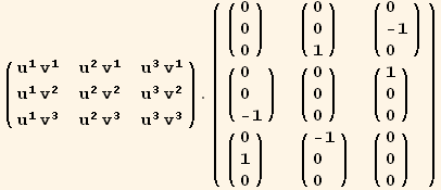
As usual, there are a number of ways to calculate this in dot mode. The following is one method.
In[53]:=
![]()
![]()
![]()
![]()
![]()
![]()
![]()
![]()
![]()
Out[54]=
![]()
![]()
Out[56]=
![]()
![]()
Out[58]=
![]()
Out[60]//MatrixForm=

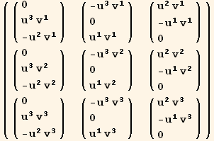
If we wish to see the extra contraction as a separate step we can pick up from the penultimate line above.
In[61]:=
![]()
![]()
![]()
![]()
![]()
![]()
![]()
Out[62]=

![]()
Out[64]//MatrixForm=
![]()
Out[66]//MatrixForm=

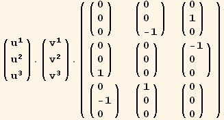
(When MatrixForm is the head of an expression it is transparent to operations.) The following shows an alternative dot mode expansion of the same expression.
In[67]:=
![]()
![]()
![]()
![]()
![]()
![]()
![]()
![]()
![]()
![]()
![]()
Out[68]=
![]()
![]()
Out[70]=
![]()
![]()
Out[72]=
![]()
Out[74]=

![]()
Out[76]//MatrixForm=

4. Order of the Final Free Indices
We have to keep an eye on the desired order of the final free indices. Consider the following expression.
In[77]:=
![]()
![]()
Out[77]=
![]()
Out[78]=

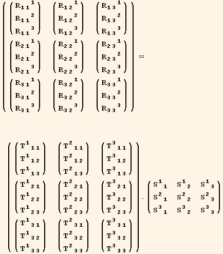
When we do this in the dot mode we must be certain that the levels of the final array correspond to the levels of the left hand side.
In[79]:=
![]()
![]()
![]()
![]()
![]()
![]()
![]()
![]()
![]()
![]()
![]()
![]()
Out[80]=
![]()
![]()
Out[82]=
![]()
![]()
Out[84]=
![]()
Out[86]=

![]()
Out[88]=

Out[89]=
![]()
The final transposition tests our knowledge of the Transpose command. We want {b,c,a} to go into positions {2,3,1} to give {a,b,c}.
More Practice with Array Calculations
The following provides some more practice in the array manipulation of tensors.
1. Contracting two vectors
The following is the Tensorial contraction of two vectors.
In[90]:=
![]()
![]()
Out[90]=
![]()
Out[91]=
![]()
This can be done as a dot mode calculation as follows...
In[92]:=
![]()
![]()
![]()
![]()
Out[92]=
![]()
Out[93]=
![]()
Out[94]=

Out[95]//MatrixForm=
![]()
We could also generate the outer product of u and v and then contract on the two levels. However, this is inefficient because it generates extra terms that are then thrown away.
In[96]:=
![]()
![]()
Out[96]//MatrixForm=

Out[97]=
![]()
In[98]:=
![]()
![]()
Out[98]//MatrixForm=

Out[99]=
![]()
2. Contracting a vector on a 2nd order tensor
We can contract a vector on either slot of a 2nd order tensor. In tensor indicial expressions the factors can appear in any order. Here we contract u on the second index of T. Contracting a second order tensor on a vector gives us a vector.
In[100]:=
![]()
![]()
Out[100]=
![]()
Out[101]//MatrixForm=

The following uses a dot mode calculation.
In[102]:=
![]()
![]()
![]()
![]()
Out[102]=
![]()
Out[103]=
![]()
Out[104]=

Out[105]//MatrixForm=

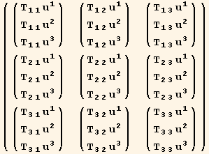
We can also form the tensor product of T and u with Outer and then contract using ContractArray on the 2nd and 3rd slots or levels. Notice again that many extra unused terms are generated.
In[106]:=
![]()
![]()
Out[106]//MatrixForm=
Out[107]//MatrixForm=

If we contract the vector on the first index we obtain...
In[108]:=
![]()
![]()
Out[108]=
![]()
Out[109]//MatrixForm=

which is definitely different than contracting on the second slot. In the dot mode this becomes...
In[110]:=
![]()
![]()
![]()
![]()
Out[110]=
![]()
Out[111]=
![]()
Out[112]=

Out[113]//MatrixForm=

Notice that we didn't have to do any transpositions of levels. Tensorial automatically made j the lower level in the T array because it comes after i in sort order.
In the following we take the outer product T⊗u and keep a strict slot order by using an ascending set of indices. Then we want to contract the resulting array on the first and third slots.
In[114]:=
![]()
![]()
Out[114]//MatrixForm=

Out[115]//MatrixForm=

3. Contractions of two 2nd order tensors
We have four choices on how two second order tensors can be contracted. In addition, there are two ways to perform a full contraction to obtain a scalar.
Single contractions
The following are the four possible single contractions of S⊗T performed in index mode.
In[116]:=
![]()
![]()
![]()
Out[116]=
![]()
Out[117]=

In[119]:=
![]()
![]()
![]()
Out[119]=
![]()
Out[120]=

In[122]:=
![]()
![]()
![]()
Out[122]=
![]()
Out[123]=

In[125]:=
![]()
![]()
![]()
Out[125]=
![]()
Out[126]=

Calculating S⊗T...
In[128]:=
![]()
Out[128]//MatrixForm=

and performing the contractions on the various slots.
In[129]:=
![]()
![]()
Out[129]//MatrixForm=

Out[130]=
![]()
In[131]:=
![]()
![]()
Out[131]//MatrixForm=

Out[132]=
![]()
In[133]:=
![]()
![]()
Out[133]//MatrixForm=

Out[134]=
![]()
In[135]:=
![]()
![]()
Out[135]//MatrixForm=

Out[136]=
![]()
Calculating the same contractions in dot mode.
In[137]:=
![]()
![]()
![]()
![]()
![]()
Out[137]=
![]()
Out[138]=
![]()
Out[139]=

Out[140]=

Out[141]=
![]()
In[142]:=
![]()
![]()
![]()
![]()
![]()
Out[142]=
![]()
Out[143]=
![]()
Out[144]=

Out[145]=

Out[146]=
![]()
In[147]:=
![]()
![]()
![]()
![]()
![]()
Out[147]=
![]()
Out[148]=
![]()
Out[149]=

Out[150]=

Out[151]=
![]()
In[152]:=
![]()
![]()
![]()
![]()
![]()
Out[152]=
![]()
Out[153]=
![]()
Out[154]=

Out[155]=

Out[156]=
![]()
Double contractions
The following are the two double contractions of S⊗T.
In[157]:=
![]()
![]()
Out[157]=
![]()
Out[158]=
![]()
In[159]:=
![]()
![]()
Out[159]=
![]()
Out[160]=
![]()
Doing the same calculation by contracting the outer product array calculated in the previous section.
In[161]:=
![]()
![]()
Out[161]=
![]()
Out[162]=
![]()
In[163]:=
![]()
![]()
Out[163]=
![]()
Out[164]=
![]()
Doing the same calculations in dot mode.
In[165]:=
![]()
![]()
![]()
![]()
![]()
Out[165]=
![]()
Out[166]=
![]()
Out[167]=

Out[168]//MatrixForm=
![]()
Out[169]=
![]()
In[170]:=
![]()
![]()
![]()
![]()
![]()
Out[170]=
![]()
Out[171]=
![]()
Out[172]=

Out[173]//MatrixForm=
![]()
Out[174]=
![]()
4. Contracting a 3rd order tensor with a 2nd order tensor
With a 2nd and 3rd order tensor we have many possiblities for contraction. Let's just do one case of a double contraction.
In[175]:=
![]()
![]()
Out[175]=
![]()
Out[176]//TableForm=
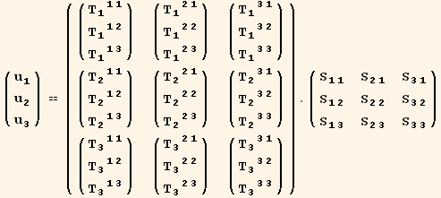
Performing the same calculation in dot mode...
In[177]:=
![]()
![]()
![]()
![]()
![]()
Out[177]=
![]()
Out[178]=
![]()
Out[179]=
Out[180]=

Out[181]=
![]()
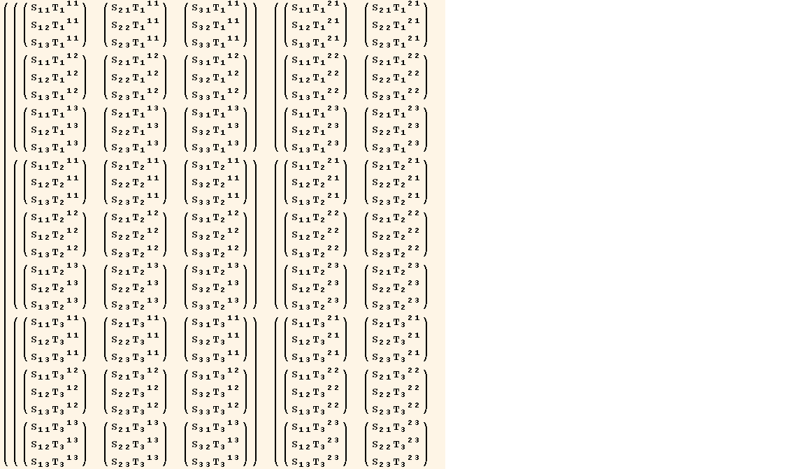
Constructing T⊗S and contracting...
In[182]:=
![]()
![]()
![]()
Out[182]//MatrixForm=
Out[183]//MatrixForm=

Out[184]=
![]()
5. Sometimes Mathematica Array Methods Are Better
If we wanted to calculate the determinant of a tensor with the following values...
In[185]:=
![]()
We could expand the tensor and use the Mathematica Det function.
In[186]:=
![]()
Out[186]=
![]()
Or we could calculate using the Levi-Civita symbol and Tensorial methods.
In[187]:=
![]()
and then evaluate the determinant by tensor methods. We obtain the same answer.
In[188]:=
![]()
![]()
Out[188]=
![]()
Out[189]=
![]()
The array method is approximately 3 times faster.
In[190]:=
![]()
![]()
Out[190]=
![]()
Out[191]=
![]()
In[192]:=
![]()
![]()
| Created by Mathematica (November 22, 2007) |