index.html

Continuum Mechanics

Renan Cabrera
cabrer7@uwindsor.ca
Physics Department
University of Windsor
Ontario Canada

This notebook presents an application in Continuum Mechanics, based in the classic Landau's book Elasticity Theory. A much more comprehensive application was done by Jean-Francois in his package Continuum Mechanics.

Initialization

In[1]:=

There is one animation at the beginning of The strain tensor section that requires the DrawGraphics package. If you don't have that package you can skip the animation.

In[2]:=

In[4]:=

In[5]:=

In[6]:=

In[7]:=

In[8]:=

In[9]:=

Forcing the identity in order to improve the efficiency of the computation

In[12]:=

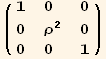
Metric in Euclidean Cylindrical Coordinates

Defining an Euclidean metric in cylindrical coordinates

In[13]:=

$(metric = DiagonalMatrix[{1, ρ^2, 1}])//MatrixForm$

Out[13]//MatrixForm=

$( {{1, 0, 0}, {0, ρ^2, 0}, {0, 0, 1}} )$

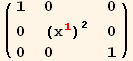
In[14]:=

Out[14]//MatrixForm=

$( {{1, 0, 0}, {0, (x_1^1)^2, 0}, {0, 0, 1}} )$

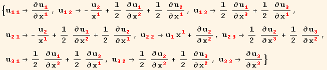
Calculating the Christoffel symbols from the metric

In[16]:=

In[17]:=

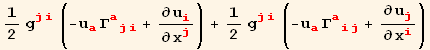
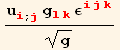
The strain tensor = (+)

The strain tensor is related to the change in the distance between two generic points when they are subject to a displacement. The following amimation shows this distance represented by a the blue vector. (Select and evaluate the thin closed cell for the animation.)

[Graphics:HTMLFiles/index_26.gif]

The strain tensor could be calculated in terms of the covariant derivatives of the displacement vector

In[27]:=

ExpandedStrainTensorRule = udd[red[i_], red[j_]] →ToFlavor[red][1/2 (CovariantD[ud[i], j] + CovariantD[ud[j], i])]

Out[27]=

An explicit expansion of the strain tensor in cylindrical coordinates is

In[28]:=

Out[28]=

-1/2 u_a^a Γ_ (aij)^(aij) - 1/2 u_a^a Γ_ (aji)^(aji) + 1/2 ∂u_i^i/∂x_j^j + 1/2 ∂u_j^j/∂x_i^i

Out[29]=

where we stored the values in a rule associated to the stress tensor

In[31]:=

Out[31]=

A comparison with the result found in Landau's book reveals that they are different. They are different because Landau works with the so called "physical components" and here we work with either contravariant of covariant components.

In a next section we are going to need an explicit expression for the divergence of the displacement

In[32]:=

Out[32]=

Out[33]=

1/2 g_ (ji)^(ji) (-u_a^a Γ_ (aji)^(aji) + ∂u_i^i/∂x_j^j) + 1/2 g_ (ji)^(ji) (-u_a^a Γ_ (aij)^(aij) + ∂u_j^j/∂x_i^i)

Out[34]=

u_ (b_Symbolb_Symbol)^(b_Symbolb_Symbol) →u_1^1/x_1^1 + ∂u_1^1/∂x_1^1 + ∂u_2^2/∂x_2^2/(x_1^1)^2 + ∂u_3^3/∂x_3^3

Compatibility equations =0

The definition of the stress tensor does not allow to calculate the displacements given the values of the stress tensor by itself. More equations are needed to constrain the six values of the stress tensor.

The compatibility equations in cylindrical coordinates are such that each term of the following array must be zero. Only three of them are independent. This operation may take more than a few seconds.

In[35]:=

stepa = CovariantD[ℰdd[red @ i, red @ j], {red @ k, red @ l}] * εuuu[red @ i, red @ k, red @ m] * εuuu[red @ j, red @ l, red @ n]

Out[35]=

Out[36]=

Thermodynamic potentials

Three thermodynamical potentials can be defined in terms of the stress tensor

Internal Energy

Helmholtz Free Energy

Gibbs Energy

Free energy expansion for isotropic materials in terms of the Lamé moduli μ and λ

In[37]:=

In[38]:=

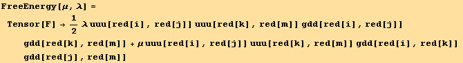
Out[38]=

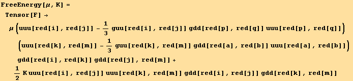
The (generalized) trace describes a pure Hydrostatic compression

In[39]:=

Out[39]=

The traceless part of the strain tensor describes a pure shear stress

In[40]:=

Out[40]=

Hooke's Law

Hooke's Law is obtained from the free energy expansion for isotropic materials (in terms of μ and the Hydrostatic modulus K) applied to the equilibrium equation

In[41]:=

Out[41]=

The stress tensor can be found taking the partial derivative of the Free energy respect to the strain tensor =.

The metric is independent of the displacement

In[42]:=

Metric simplifying the entire expression and using TensorSimplify.

In[43]:=

$DisplayForm[FrameBox[IsotropicStressTensorRule = σdd[red[r_], red[s_]] →Collect[SimplifyTensorSum[TensorSimplify[%]/. {gdu[b_, b_] →3, gud[b_, b_] →3}], {μ}]]]$

Out[43]=

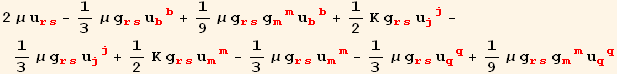
Out[44]//DisplayForm=

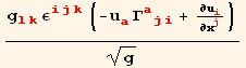
Equilibrium Equation

The equilibrium equation that comes from Newtons's Law is +ρ ==0.

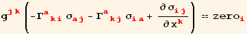
Neglecting the volume forces we have only the first term. It is convenient to expand in terms of the covariant indices of the stress tensor, so the equilibrium equation becomes

In[45]:=

Out[45]=

The zero tensor balances the free index on both sides of the equation, behaves as a zero, and expands to a zero array. Expanding and expressing the stress tensor in terms of the strain tensor as first step

In[46]:=

Out[46]=

Out[47]=

g_ (jk)^(jk) (-Γ_ (aki)^(aki) σ_ (aj)^(aj) - Γ_ (akj)^(akj) σ_ (ia)^(ia) + ∂σ_ (ij)^(ij)/∂x_k^k) == zero_i^i

Out[49]=

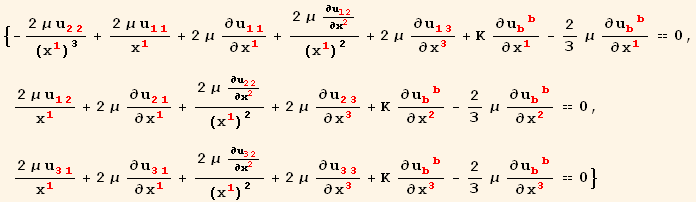
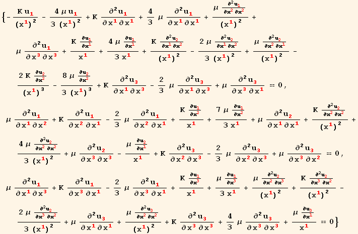
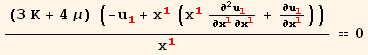
and finally we obtain the homogeneous equation for the displacement in cylindrical coordinates

In[50]:=

Out[50]=

Example1: Cylindrical tube under an internal constant hydrostatic pressure

This is an example solved in Landau's book Elasticity Theory. Chapter 7 problem 4

Using the expression of the deformation in cylindrical coordinates. The deformation depends only on the radial coordinate so we define the rule

In[51]:=

$ConditionExample1 = {PartialD[_][_, xu[i : red[2] | red[3]]] →0, PartialD[_][_, HoldPattern[{___, Tensor[x, {red[2] | red[3]}, {Void}], ___}]] →0}$

Out[51]=

${PartialD[_][_, x_ (i : 2 | 3)^(i : 2 | 3)] →0, PartialD[_][_, HoldPattern[{___, x_ (2 | 3)^(2 | 3), ___}]] →0}$

which simplifies the equilibrium equations to

In[52]:=

Out[52]=

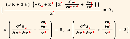
Paying attention to the first equilibrium equation we realize that it is an ODE (Ordinary Differential Equation) that can be easily solved

In[53]:=

Out[53]=

((3 K + 4 μ) (-u_1^1 + x_1^1 (x_1^1 ∂^2u_1^1/∂x_1^1∂x_1^1 + ∂u_1^1/∂x_1^1)))/x_1^1 == 0

Out[54]=

Out[55]=

Out[56]=

${u_1^1→C[3]/x_1^1 + C[4] x_1^1, u_2^2→0, u_3^3→0}$

Alternatively, we can use the new feature of Tensorial 4.0, a copy paste , to solve the differential equation of the first equilibrium equation

In[57]:=

Out[57]=

Out[58]=

Out[59]=

Out[60]=

${u_1^1→C[3]/x_1^1 + C[4] x_1^1, u_2^2→0, u_3^3→0}$

The remaining two equilibrium equations are zero as it shown in the next subsection.

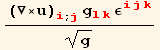
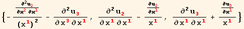
Curl of the Curl of the Displacement

In[61]:=

Out[61]=

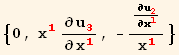
The curl of the displacement tensor is

In[62]:=

Out[62]=

(u_i^i_ (; j) g_ (lk)^(lk) ε_ (ijk)^(ijk))/g^(1/2)

Out[63]=

(g_ (lk)^(lk) ε_ (ijk)^(ijk) (-u_a^a Γ_ (aji)^(aji) + ∂u_i^i/∂x_j^j))/g^(1/2)

Out[64]=

${0, x_1^1 ∂u_3^3/∂x_1^1, -∂u_2^2/∂x_1^1/x_1^1}$

Defining a special display format for Curlu, and taking the curls once more on top of our previous result:

In[66]:=

Taking the curls once more on the top of our previous result

In[67]:=

Out[67]=

((∇×u)_i^i_ (; j) g_ (lk)^(lk) ε_ (ijk)^(ijk))/g^(1/2)

Out[68]=

-((∇×u)_a^a g_ (lk)^(lk) Γ_ (aji)^(aji) ε_ (ijk)^(ijk))/g^(1/2) + (g_ (lk)^(lk) ε_ (ijk)^(ijk) ∂(∇×u)_i^i/∂x_j^j)/g^(1/2)

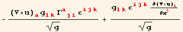
Out[69]=

Out[70]=

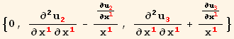
${0, ∂^2u_2^2/∂x_1^1∂x_1^1 - ∂u_2^2/∂x_1^1/x_1^1, ∂^2u_3^3/∂x_1^1∂x_1^1 + ∂u_3^3/∂x_1^1/x_1^1}$

which are proportional to the remaining two equilibrium equations. The curl is interpreted as the measure of an infinitesimal rotation. A static cylinder under hydrostatic pressure does not generate rotations, so the last two equilibrium equations are identical to zero.

The conditions of a relative pressure p inside the tube defines the values of the constants

In[71]:=

$ConstantsC4C3 = {C[4] → (p r^2 (1 + σ) (1 - 2 σ))/((R^2 - r^2) "E"), C[3] → (p r^2 R^2 (1 + σ))/((R^2 - r^2) "E")}$

Out[71]=

${C[4] → (p r^2 (1 - 2 σ) (1 + σ))/(E (-r^2 + R^2)), C[3] → (p r^2 R^2 (1 + σ))/(E (-r^2 + R^2))}$

where E and σ are the Young and Poisson moduli that are easier to measure in the experiment

Calculation of the Strain tensor

In[72]:=

Out[72]=

In our case the Strain tensor is

In[73]:=

Out[73]=

The divergence of the displacement tensor (trace of the strain tensor) is

In[75]:=

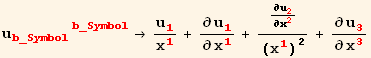
TraceTubeStrainRule = udu[red[b_], red[b_Symbol]] →%/.DisplacementDivergenceRule/.SolDisplacement/.ConstantsC4C3

Out[75]=

Out[76]=

The following rule defines the Lame moduli in terms of the Young Poisson moduli.

In[77]:=

Out[77]=

Calculating the Stress Tensor

From the previous parts we get everything necessary to calculate the Stress Tensor

In[78]:=

TubeStressTensor = Simplify[ArrayExpansion[red[i], red[j]][%]/.u→TubeStrain/.TensorValueRules[TubeStrain]/.ToPoissonYoung]

Out[78]=

Out[79]=

Out[80]=

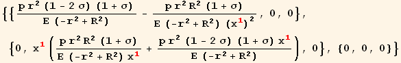
${{(p r^2 (R^2 - (x_1^1)^2))/((r^2 - R^2) (x_1^1)^2), 0, 0}, {0, -(p r^2 (R^2 + (x_1^1)^2))/(r^2 - R^2), 0}, {0, 0, -(2 p r^2 σ)/(r^2 - R^2)}}$

which agrees with Landau's solution after is divided by the square of . This is because Landau uses the physical components instead of the covariant components as we use here.

Created by Mathematica (November 22, 2007)