Relativistic Quantum Mechanics: Dirac Equation
Renan Cabrera
cabrer7@uwindsor.ca
Initialization
In[1]:=
![]()
In[2]:=
![]()
In[3]:=
![]()
In[4]:=
![]()
![]()
In[6]:=
![]()
![]()
Dirac's Gamma
First let's define the α matrices directly from the Pauli matrices
In[8]:=

In[9]:=
![]()
![]()
Out[9]=
![]()
Out[10]=
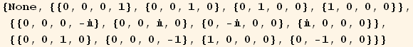
We also need β
In[11]:=
![]()
Out[11]=
![]()
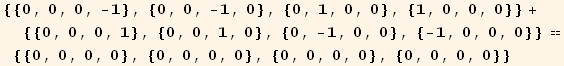
They anticommute
In[12]:=
![]()
![]()
Out[12]=
![]()
Out[13]=
In[14]:=
![]()
![]()
![]()
Out[14]=
![]()
Out[15]=
Out[16]=
![]()
The following cell illustrates the commutation relation in detail. Just set the index equal to 1,2 or 3.
In[17]:=
![]()
![]()
![]()
![]()
![]()
![]()
![]()
Out[18]=
![]()
![]()
Out[20]=
Out[21]=
Out[22]=
![]()
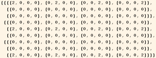
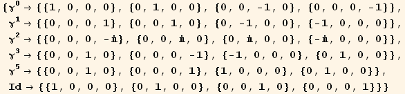
The convenient Dirac's Gamma are defined from the α and β matrices suitable for the metric we defined.(other shapes of the metric would require silight changes)
In[24]:=
![]()
But it is also useful to define more components for γ and the identity matrix
In[25]:=

Out[25]=
In[26]:=
![]()
![]()
In[27]:=
![]()
![]()
Out[27]=
![]()
Out[28]=
![]()
Dirac Equation
Now let's define the Dirac Spinor ψ
In[29]:=
![]()
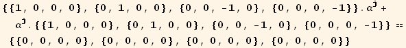
Then The Dirac equation is:
In[30]:=
![]()
![]()
Out[30]=
![]()
Adding some additional rules.
In[32]:=
![]()
![]()
![]()
![]()
![]()
![]()
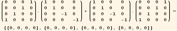
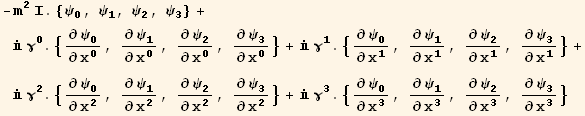
The Dirac equation with the coordinates explicitly:
In[38]:=
![]()
Out[38]=
![]()
where m is the mass and its sign can be either positive or negative. Dirac interpretations says that they represent a particle and its antiparticle.
Expanding over the γ 's
In[39]:=
![]()
Out[39]=
![]()
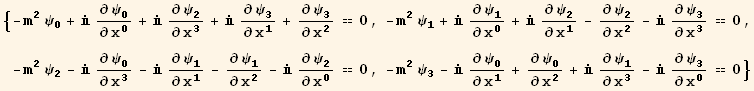
Expanding and replacing values we get the following system of first order partial differential equations.
In[40]:=
![]()
![]()
Out[40]=
Out[41]=
Particle in the Rest Frame
In[42]:=
![]()
Out[42]=

Let P to be the 4momentum vector. Let's try a solution for a free particle in a rest frame system. This means that the only component of the momentum that survives is the zero one.
In[43]:=
![]()
![]()
Out[43]=
![]()
Where we define the tensor object c as a constant. The same for the components of the momentum and we format the zero component as E refering as the enegy.
In[45]:=
![]()
![]()
![]()
![]()
Plugging in this trial solution into the actual Dirac equation we get.
In[49]:=
![]()
![]()
Out[49]=
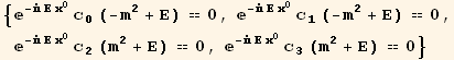
Out[50]=
![]()
And after some simplification:
In[51]:=
![]()
Out[51]=
![]()
The system has a non trivial solution only if the determinat is zero. (Not all the equations are independent)
In[52]:=
![]()
Out[52]=
![]()
If we let the Energy or ![]() to be a free parameter we get two solutions that will make the determinant zero.
to be a free parameter we get two solutions that will make the determinant zero.
In[53]:=
![]()
Out[53]=
![]()
One corresponds to a positive energy (particle?)and the other to a negative energy (antiparticle?)
In[54]:=
![]()
Out[54]=
![]()
Recalling the trial solution, this means that the solutions are four; the first two corresponding to the positive energy.
In[55]:=
![]()
Out[55]=
![]()
In[56]:=
![]()
Out[56]=
![]()
And the last two corresponding to the negative energy
In[57]:=
![]()
Out[57]=
![]()
In[58]:=
![]()
Out[58]=
![]()
Free Particle Solution
Let P to be the 4momentum vector. Let's try a solution for the free particle with the following plane wave.
In[59]:=
![]()
Out[59]=
![]()
Where we define the tensor obejct c as a constant. The same for the components of the momentum.
In[60]:=
![]()
![]()
![]()
![]()
![]()
Plugging in this trial solution into the actual Dirac equation we get.
In[65]:=
![]()
Out[65]=
![]()
In[66]:=
![]()
![]()
![]()
Out[66]=
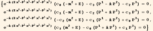
Out[67]=
![]()
Out[68]=
![]()
And after some simplification:
In[69]:=
![]()
Out[69]//MatrixForm=
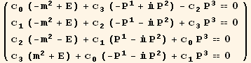
Extracting a matrix from the system of equations
In[70]:=
![]()
Out[70]=
![]()
The system has a non trivial solution only if the determinant is zero. (Not all the equations are independent)
In[71]:=
![]()
Out[71]=
![]()
If we let the Energy or ![]() to be a free parameter we get two solutions that will make the determinat zero.
to be a free parameter we get two solutions that will make the determinat zero.
In[72]:=
![]()
Out[72]=
![]()
With positive and negative possibilities for the energy.
There are only two different eigenvalues, this means that for each one there is a 2D plane space, included into the original 4D space. In other words for each energy we can choose two arbitrary parameters to span a 2D plane and we can choose any pair of equations to solve the parameters provided that a the particular pair of equations are not parallel (linearly dependent)
I played numerically with the equations and it seems that no pair of equations are ever parallel for any case of the autovalues, but conventionally there is a particular way to choose them as follows.
For the positive energy:
In[73]:=
![]()
![]()
Out[73]=
![]()
Out[74]=
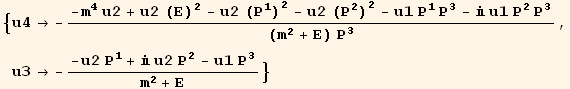
The first eigenvector is:
In[75]:=
![]()
Out[75]=
![]()
The second eigenvector is:
In[76]:=
![]()
Out[76]=
![]()
Now for the eigenvectors of negative energy
In[77]:=
![]()
![]()
Out[77]=
![]()
Out[78]=
![]()
In[79]:=
![]()
Out[79]=
![]()
In[80]:=
![]()
Out[80]=
![]()
References
1) Kane, Gordon. Modern Elementary Particel Physics. (1993) Addison-Wesley. Section 5.1
2) Greiner, Walter & Reinhardt, Jochim. Field Quantization. (1996) Springer. Section 5
3) Doughty, Noel E. Lagrangian Interaction. (1990) Addison-Wesley Section 20.3
| Created by Mathematica (November 22, 2007) |