index.html

Flat and Curved

Coordinate Transformation of the Flat Plane and the Hyperbolic Half-Plane

David Park
djmp@earthlink.net
http://home.earthlink.net/~djmp/

This example illustrates a number of features of Tensorial. It shows how Tensorial melds with the standard notebook interface and ordinary Mathematica. With Tensorial it is possible to follow and reproduce textbook or research paper derivations and calculations. More importantly, it is possible to combine discursive text with interactive calculations, graphics and animation to produce clear, informative and even elegant documents.

In this notebook we examine a coordinate transformation of the flat plane, and another description of a plane that is not flat. These are both adaptations of Problems in Gravitation by James Hartle. In some places I have done the expositions in some detail and sometimes by alternative paths both to illustrate various features of Tensorial and to show that expositions can be presented at various levels of detail and can follow textbook styles.

Initiation

In[8]:=

The DrawGraphics package is needed for the graphics in this notebook. It can be obtained on the Mathematica page of my web site above. Or you can skip the graphics.

In[9]:=

In[10]:=

Here we declared two additional flavors of indices and in DeclareBaseIndices we associated different base index symbol sets with the different flavors. This will allow our various tensor quantities to display with their corresponding coordinate labels. This is part of the multibase capability of Tensorial 4.0.

Flat

A coordinate transformation on the Cartesian plane does not change the flatness of the plane. Let's explore this using the coordinate transformation given in Hartle Problem 2.7. We will use regular black indices to represent xy coordinates and red indices to represent the μν coordinates given below.

Coordinate Transformation

Here we use tensor notation and Mathematica's functional ability to represent and implement a coordinate transformation in a generic manner.

In[15]:=

Out[16]=

Out[18]=

Out[19]=

${x_x^x[x_μ^μ, x_ν^ν], x_y^y[x_μ^μ, x_ν^ν]}$

Out[21]=

Next, we can actually set the coordinate functions. Since they are functions we use the Mathematica Function expression.

In[22]:=

$SetTensorValueRules[xu[a], {Function[{μ, ν}, μ ν], Function[{μ, ν}, 1/2 (μ^2 - ν^2)]}]$

Out[23]=

${x_x^x→Function[{μ, ν}, μ ν], x_y^y→Function[{μ, ν}, 1/2 (μ^2 - ν^2)]}$

In the following we use the coordinates as ordinary elements on the left and as functions on the right. Nothing more clearly illustrates that coordinates are basically functions but we tend to use them both as functions and as quantities that can have ordinary values.

In[24]:=

Out[25]=

${x_x^x, x_y^y} == {x_x^x[x_μ^μ, x_ν^ν], x_y^y[x_μ^μ, x_ν^ν]}$

Out[27]=

${x_x^x, x_y^y} == {x_μ^μ x_ν^ν, 1/2 ((x_μ^μ)^2 - (x_ν^ν)^2)}$

Out[29]=

${x, y} == {μ ν, 1/2 (μ^2 - ν^2)}$

Out[30]//TableForm=

x==μ ν

We can write a μν parametrization for a point in the xy plane.

In[31]:=

Out[31]=

${μ ν, 1/2 (μ^2 - ν^2)}$

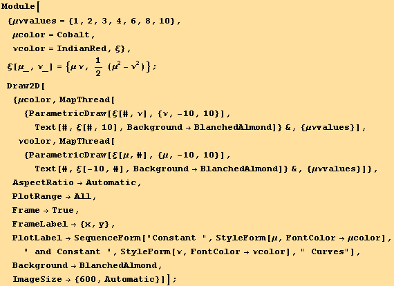
We can then plot and label two sets of coordinate curves in the xy plane.

In[32]:=

[Graphics:HTMLFiles/index_42.gif]

In[33]:=

Coordinate Basis Vectors, Orthonormal Basis Vectors and the Metric

Coordinate basis vectors are defined as the rate of change of a point in the plane with respect to each of the coordinates. The following calculates and sets the coordinate basis vectors in the red (μν) coordinate system.

In[34]:=

Print[The a'th coordinate basis vector is the rate of change of the point  in the xy plane with respect to the a'th coordinate]

$%%//UseCoordinates[{μ ν, 1/2 (μ^2 - ν^2)}]//Simplify$

Out[35]=

Out[37]=

Out[39]=

$e_a^a == {∂x_x^x/∂x_a^a, ∂x_y^y/∂x_a^a}$

Out[41]=

${e_μ^μ == {∂x_x^x/∂x_μ^μ, ∂x_y^y/∂x_μ^μ}, e_ν^ν == {∂x_x^x/∂x_ν^ν, ∂x_y^y/∂x_ν^ν}}$

Out[43]=

Out[44]=

${e_μ^μ == {ν, μ}, e_ν^ν == {μ, -ν}}$

Out[46]=

Out[48]=

${e_μ^μ→ {x_ν^ν, x_μ^μ}, e_ν^ν→ {x_μ^μ, -x_ν^ν}}$

In the first line above, note that the free index a is balanced on both sides of the equation because an up index in the denominator of a partial is the same as a down index in the expression. However, in the second line we have something of an 'improper' expression because b is not a balanced free index. This is because an individual basis vector is really an array. We have to expand the right hand side into an array, using ArrayExpansion, to reestablish an equation balanced in the free indices. I hope the rest of the calculation is straight forward. We substituted coordinate values, using UseCoordinates, to evaluate the partial derivatives, and then converted the final expressions back to indexed coordinates.

Here is a second path to calculating the coordinate basis vectors. In this path we keep the idea of coordinate functions, which we reestablish for the black coordinates.

In[49]:=

$SetTensorValueRules[xu[a], {Function[{μ, ν}, μ ν], Function[{μ, ν}, 1/2 (μ^2 - ν^2)]}]$

Out[50]=

${x_x^x→Function[{μ, ν}, μ ν], x_y^y→Function[{μ, ν}, 1/2 (μ^2 - ν^2)]}$

In[51]:=

Print[The a'th coordinate basis vector is the rate of change of the point  in the xy plane with respect to the a'th coordinate.]

Out[52]=

Out[54]=

Out[56]=

Out[58]=

Out[60]=

$e_a^a == {x_ν^ν δ_ (μa)^(μa) + x_μ^μ δ_ (νa)^(νa), x_μ^μ δ_ (μa)^(μa) - x_ν^ν δ_ (νa)^(νa)}$

Out[62]=

Out[64]=

${e_μ^μ == {x_ν^ν, x_μ^μ}, e_ν^ν == {x_μ^μ, -x_ν^ν}}$

This gives us the same expressions as the previous derivation. Notice that I used a Tensorial 'trick' to evaluate the Kroneckers. The up/down versions of the metric tensor are the same as Kroneckers and the MetricSimplify routine has definitions to carry out the simplification for base indices. We just make believe that the Kroneckers are metric tensors.

In[65]:=

We can check that the basis vectors, which point along the coordinate lines, are orthogonal.

In[66]:=

Out[66]=

Out[67]//MatrixForm=

$( {{e_μ^μ . e_μ^μ, e_μ^μ . e_ν^ν}, {e_ν^ν . e_μ^μ, e_ν^ν . e_ν^ν}} )$

Out[68]//MatrixForm=

$( {{μ^2 + ν^2, 0}, {0, μ^2 + ν^2}} )$

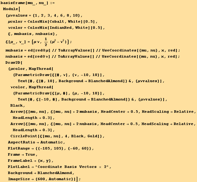
This is, in fact, the definition of the metric tensor. The fact that it is diagonal means that the two coordinate basis vectors are orthogonal. We can actually look at the basis vectors in the following animation that moves the coordinate basis along the μ==6 coordinate line.

In[69]:=

FrontEndExecute[{FrontEnd`SelectionAnimate[200, AnimationDisplayTime→0.1, AnimationDirection→ForwardBackward]}]

[Graphics:HTMLFiles/index_118.gif]

In the above plot the vectors were represented at twice their normal length just so they would look better. We see that as they move toward the origin the basis vectors change in length. The vectors are orthogonal, but not orthonormal because they are not unit or even constant length.

We can set the metric tensor values from the metric tensor computed above. We have to convert the coordinate symbols to indexed coordinates.

In[74]:=

Out[76]=

Sometimes we may wish to generate an orthonormal basis. To do this, we need to calculate the transformation matrix, Λ, from a coordinate basis to an orthonormal basis. We will represent the orthonormal basis in blue. The routine, OrthonormalTransformation calculates the transformation matrix. (See the Help page for OrthonormalBasis.)

In[77]:=

Out[77]=

${{1/(μ^2 + ν^2)^(1/2), 0}, {0, 1/(μ^2 + ν^2)^(1/2)}}$

We set values for the Λ transformation matrix in the last statement. In the following statements we use it to transform the basis vectors from the red coordinate frame to the blue orthonormal frame. Notice that transformation matrices are always up-down indexed objects with different flavors for the indices. (To reverse the flavors, take the inverse of the matrix.) When carrying out a transformation of some element we simply have to match the flavors and indices to obtain a consistent expression.

In[79]:=

Out[79]=

Out[80]=

We can check that these basis vectors are actually orthonormal.

In[82]:=

Out[82]=

Out[83]//MatrixForm=

$( {{e_μ^μ . e_μ^μ, e_μ^μ . e_ν^ν}, {e_ν^ν . e_μ^μ, e_ν^ν . e_ν^ν}} )$

Out[84]//MatrixForm=

Alternatively, we can calculate the metric in the blue basis by transforming the metric in the red basis. We need a transformation for each index.

In[85]:=

Out[85]=

Out[86]=

$( {{g_ (μμ)^(μμ), g_ (μν)^(μν)}, {g_ (νμ)^(νμ), g_ (νν)^(νν)}} ) == ( {{1, 0}, {0, 1}} )$

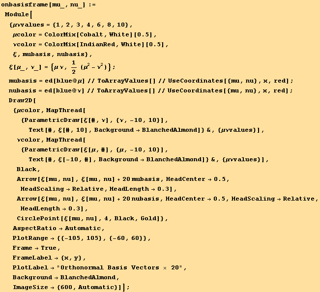
An animation of the orthonormal basis illustrates that the basis vectors are always unit length.

In[87]:=

FrontEndExecute[{FrontEnd`SelectionAnimate[200, AnimationDisplayTime→0.1, AnimationDirection→ForwardBackward]}]

[Graphics:HTMLFiles/index_191.gif]

Notice that a low range of values for the μν coordinates encompass a much wider range of values for the xy coordinates, which is why we had to scale up the basis vectors by a factor of 20 to obtain a good view. Using graphics to accompany derivations and expositions can be an immense aid. One can't make the graphic unless one has a working, calculational knowledge of the material, so producing a good working graphic is a good test both of the theory and one's knowledge of it.

Line Element, Geodesic Equation and Curvature Elements

Continuing on with definitions established in the previous section, we can write the line element for the plane in μν coordinates. As a part of our development we will use the fact that the metric tensor is symmetrical. We can declare that symmetry with the following statement.

In[92]:=

Out[92]=

In[93]:=

Out[94]=

Out[96]=

Out[98]=

Out[100]=

The symmetry of the metric was actually built into its stored values, and ultimately traces back to the symmetry of dot products, so we could have skipped the penultimate line above.

In Hartle's problem 2.7 he establishes the flatness of the space in μν coordinates by calculating the ratio of the circumference to the radius of a circle. Let's follow a different path and calculate a geodesic in μν coordinates and demonstrate that it is a straight line.

The first step is to calculate and store the Christoffel symbols that tell us how vectors at one location are 'connected' to vectors at a nearby location. We do that with the following statement. The second statement displays the independent up Christoffel symbols. Since the Christoffel symbols are symmetric in the last two indices we only display the values for which the last two indices are ordered.

In[101]:=

MapThread[SetTensorValueRules[#1, #2] &, {{Γddd[a, b, c], Γudd[a, b, c]}//ToFlavor[red], CalculateChristoffels[labs, red]}] ;

$SelectedTensorRules[Γ, Γudd[_, b_, c_]/;OrderedQ[{b, c}]]//UseCoordinates[{μ, ν}, x, red]//TableForm$

Out[102]//TableForm=

The geodesic equation takes the following form.

In[103]:=

Out[103]=

Is most texts the equation is simply written with a 0 on the right hand side. This is formally incorrect because the free index does not balance on each side of the equation. By declaring a 'zero' tensor we can make the free indices balance and Tensorial will automatically substitute 0's when the equation is expanded. (And Tensorial will also combine zero tensors with other tensors in the proper manner.)

Let's see if we can expand and solve this equation. Notice that when we use UseCoordinates to substitute functions of s the Tensorial differential equations morph into standard Mathematica differential equations.

In[104]:=

$diffeqns0 = Map[Distribute[Cancel[# (μ[s]^2 + ν[s]^2)]] &, %%, {2}]$

Out[105]=

Out[107]=

Out[109]=

DSolve will not directly solve these equations but we can still demonstrate that these equations give geodesics that are straight lines. We write equations for x and y in terms of μ and ν and then show that x and y depend at most only linearly on s. That is, we want to show that the second derivatives of x and y with respect to s are both zero.

In[110]:=

Out[113]=

Out[114]=

We can easily solve the geodesic equations numerically. We have to add initial conditions that give a starting point and direction for each geodesic. The following solves for a set of geodesics going through various points at various angles. We have to avoid geodesics that might go through the origin.

In[116]:=

initvals = {{1, 3, 1, 1}, {2, 3, 1, 1}, {3, 3, 1, 2}, {4, 3, 1, 1}, {6, 3, 1, 1}, {8, 3, 1, 1}, {3, 1, 1, -1}, {3, 2, 1, -1}, {3, 3, 1, -1}, {3, 4, 1, -1}, {3, 6, 1, -1}, {3, 8, -1, -1}} ;

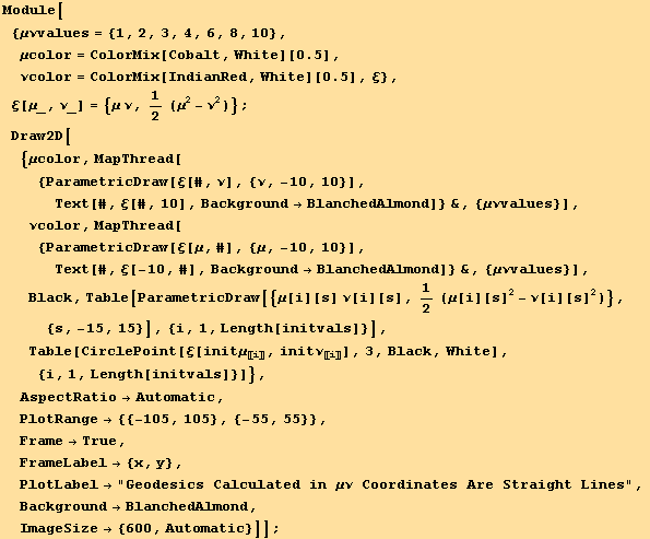
We can then plot these geodesics on top of our μν coordinate grid. To plot in the xy plane we use the parametrization {μ[s] ν[s], (-)}.

In[120]:=

[Graphics:HTMLFiles/index_293.gif]

The white points show the initial values for each of the geodesics. The geodesics are all straight lines, showing that the space is flat.

In[121]:=

We can also show that the μν metric is flat by calculating the Riemann tensor. The Riemann tensor encodes the curvature of a space and is identically zero in this case.

In[122]:=

Out[122]=

In[123]:=

Out[123]=

${g_ (ab)^(ab), g_ (ab)^(ab), e_a^a, Γ_ (abc)^(abc), Γ_ (abc)^(abc)}$

Curved

For a curved space we use the 2-dimensional metric for the hyperbolic half-plane, y>0, that Hartle gives in Problem 8.12

In[126]:=

$(cmetric = DiagonalMatrix[{1, 1}/y^2])//MatrixForm$

Out[126]//MatrixForm=

$( {{1/y^2, 0}, {0, 1/y^2}} )$

Set the metric.

In[127]:=

Out[129]=

${g_ (xx)^(xx) →1/y^2, g_ (xy)^(xy) →0, g_ (yx)^(yx) →0, g_ (yy)^(yy) →1/y^2, g_ (xx)^(xx) →y^2, g_ (xy)^(xy) →0, g_ (yx)^(yx) →0, g_ (yy)^(yy) →y^2}$

Line Element and Distance from x Axis

The line element is...

In[130]:=

Out[130]=

Out[131]=

If we travel along a line of constant x value, then dx==0 and the line element simplifies. The distance is then given by the following integral, which is divergent. We use dS==-dy since we are traveling downward.

In[132]:=

Out[132]=

If we integrate to a value ε that is greater than zero we obtain the following expression, which again diverges as ε→0.

In[133]:=

Out[133]=

Out[134]=

Geodesics

To write the geodesic equation we first have to calculate the Christoffel connection coefficients.

In[135]:=

$SelectedTensorRules[Γ, Γudd[_, a_, b_]/;OrderedQ[{a, b}]]//UseCoordinates[{x, y}]//TableForm$

Out[136]//TableForm=

We can then write down the geodesic equation and expand it using ToArrayValues[]. Now, instead of substituting {x,y} with UseCoordinates, we substitute {x[s],y[s]}. The Tensorial differential equations smoothly transistion to regular Mathematica differential equations.

In[137]:=

Out[137]=

Out[138]=

Out[139]=

${-(2 x^′[s] y^′[s])/y[s] + x^′′[s] == 0, x^′[s]^2/y[s] - y^′[s]^2/y[s] + y^′′[s] == 0}$

But there is a Killing vector ξ because the metric does not depend upon the x coordinate. The Killing vector is in the direction that leaves the metric unchanged. This provides a simplified integral of the geodesic...

In[140]:=

Out[140]=

where k is a constant. Dot products in tensor calculus are written as follows with the metric.

In[141]:=

Out[142]=

Out[143]=

x_x^x/s/(x_y^y)^2 == k

Out[144]=

Out[145]=

We can freely pick the constant k to obtain various solutions. If we pick k==0, then x will be constant and the geodesic is a vertical line. We can use the Killing equation to eliminate x'[s] from the second geodesic equation.

In[146]:=

$Eliminate[{geodesiceqns_[[2]], killingeqn}, x '[s]]$

Out[146]=

Out[147]=

Mathematica will not directly solve these equations, at least in a convenient form. We can first investigate them numerically. The Killing equation depends upon k so we can obtain a series of solutions, all passing through the same point {2,1}, for various values of k.

In[148]:=

$Do[geodesic[k][s_] = {x[s], y[s]}/.First @ NDSolve[{killingeqn, dyeqn, y '[0] == 1, x[0] == 2, y[0] == 1}, {x, y}, {s, -10, 10}], {k, 1, 5}]$

We want to draw another geodesic passing through the point {1,3}, which will not intersect any of those above.

In[150]:=

$geodesic[0][s_] = {x[s], y[s]}/.First @ NDSolve[{killingeqn, dyeqn, y '[0] == 1, x[0] == 1, y[0] == 3}/.k→0.2, {x, y}, {s, -10, 10}]$

Out[150]=

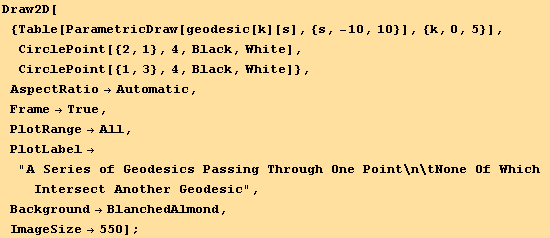
In curved space, the geodesics correspond to the 'straight' lines. In Euclidean geometry, given a line and a point outside the line, one can draw one and only one straight line through the point that does not intersect the first line. But in hyperbolic geometry we can draw many geodesics through the point that do not intersect the first geodesic.

In[151]:=

[Graphics:HTMLFiles/index_349.gif]

If we let k→0 the large geodesic will approach a vertical line.

The above numerical solutions and graphics certainly suggest that the geodesics are semicircles with their center on the x axis. Let's see if we can satisfy the geodesic equations with such solutions. The following diagram illustrates the geometry of a geodesic. (Select and evaluate the thin closed cell.)

[Graphics:HTMLFiles/index_350.gif]

There are many geodesics that can go through a point with coordinates {xp,yp}. The geodesics would have different radii r, different centers x0 and the point would be at different angles θ from the vertical point. Effectively, we obtain all the geodesics through the point from this diagram by moving the point on the half circle. But to represent them on the same plot we would have to change the scale for each geodesic because the values of xp and yp would have to remain fixed. The minimum radius will be when xp==x0. The halfcircle degenerates to a vertical line when x0-xp→∞. s[θ] is the distance of the blue point along the geodesic measured from the center (top) point of the geodesic. The distance, of course, is calculated from the metric and it is not the same as the Euclidean arc length in the diagram. Let's see how this works out.

In[153]:=

We write x and y functions that parametrize our proposed geodesic in terms of θ where we let θ be a function of distance s.

In[154]:=

Out[154]=

We substitute these in our two independent geodesic equations.

In[155]:=

Out[155]=

${x^′[s] == k y[s]^2, y^′′[s] == -k^2 y[s]^3 + y^′[s]^2/y[s]}$

Out[156]=

We can simplify the first equation, then differentiate it once to obtain a rule that we will use in the second equation.

In[157]:=

Out[157]=

Out[158]=

Out[159]//DisplayForm=

Out[160]=

The second equation is automatically satisfied if we substitute these last two expressions.

In[161]:=

Out[161]=

Out[162]=

Since, in the Killing equation k r appears as a product we can just set k==1 and solve for various r's. Take the reciprocal of the Killing equation to obtain a differential equation for distance s as a function of θ.

In[163]:=

$DSolve[{s '[θ] == 1/( r Cos[θ]), s[0] == 0}, s, θ] _[[1, 1]]$

Out[164]=

Out[165]=

Log[(Cos[θ/2] + Sin[θ/2])/(Cos[θ/2] - Sin[θ/2])]/r

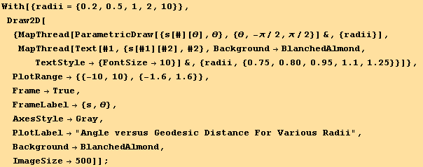
This gives us the geodesic distance s as a function of θ on each geodesic semicircle. In the following graphic we reverse the axes to show the angle as a function of s measured from the top of the semicircle.

In[167]:=

[Graphics:HTMLFiles/index_377.gif]

For a given point {xp,yp} there are two families of geodesic curves depending on whether the point lies to the left or right of the top of each semicircle. The following defines the geodesics as a function of the point, the radius and the angle from the curve top.

In[168]:=

$geodesicleft[{xp_, yp_}, r_][θ_]/;r≥yp := Module[{φ}, φ = ArcCos[yp/r] ; x0 = xp + r Sin[φ] ; {x0 - r Sin[θ], r Cos[θ]} ]$

$geodesicright[{xp_, yp_}, r_][θ_]/;r≥yp := Module[{φ}, φ = ArcCos[yp/r] ; x0 = xp - r Sin[φ] ; {x0 + r Sin[θ], r Cos[θ]} ]$

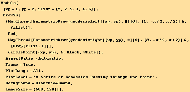
And the following plots a set of geodesics passing through {1,2} with various radii.

In[171]:=

[Graphics:HTMLFiles/index_382.gif]

Riemann and Scalar Curvature

Later, in Problem 21.11 Hartle says that the hyperbolic plane has a constant negative curvature and asks us to calculate it.

We need the Christoffel symbols set at the top of the Geodesic Equations Section. The curvature is encoded in the Riemann tensor. In Tensorial this can be calculated with the CalculateRiemannd routine, which calculates the down version of the Riemann tensor. Given the down version of the Riemann tensor and the metric, the routine CalculateRRRG will calculate the up version of the Riemann tensor, the Ricci tensor (a contraction of the Riemann tensor), the scalar curvature (a contraction of the Ricci tensor) and the Einstein tensor.

In[172]:=

Looking at the nonzero values of the up Riemann tensor and the Ricci tensor we have...

In[176]:=

Out[176]//TableForm=

The scalar curvature is a constant negative value.

In[177]:=

Out[177]=

We can check check the calculation of the scalar curvature by contracting the Ricci tensor. First we have to raise an index on the values that we have stored.

In[178]:=