6. The Fundamental Equations
of Continuum Mechanics
Initialization
![]()
![]()
![]()
![]()
![]()
![]()
![]()
![]()
![]()
![]()
![]()
![]()
The following values are taken as an example of a (red) basis frame :
![]()
![]()
![]()
![]()
![]()
![]()
![]()
![]()
![]()
and from equation (2.5) :
![]()
E (or E§) is a completely symmetric tensor :
![]()
![]()
The ChristoffelSymbol Γ is also symmetric with respect to its secons and third indices :
![]()
![]()
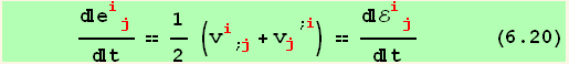
The kinematic equation have been presented in the section Strain Tensor of Chapter 2, in a non tensorial form, involving partial derivatives. Using the results of Chapter 5 on the covariant derivatives, and the fact that we have tensors, it can be easily shown that we can identify in cartesian coordinates the partial derivatives with the covariant derivatives and then see that the kinematic equations take the form
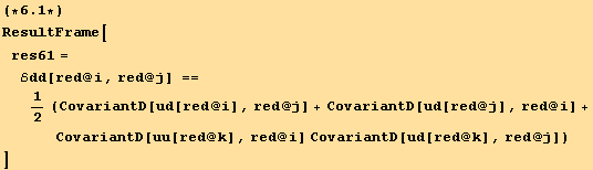
![]()
and the linear version of the kinematic equation may be written,
![(*6.2*)ResultFrame[res62 = ℰdd[red @ i, red @ j] == (ℰ§dd[red @ i_, red @ j_] = 1/2 (CovariantD[ud[red @ i], red @ j] + CovariantD[ud[red @ j], red @ i])) ]](HTMLFiles/index_29.gif)
![]()
This equation is now valid in any coordinate system. The above equation is symmetrical in its indices, but what is the meaning of the antisymmetric expression ![]() (
(![]() -
-![]() ). Consider the tensor
). Consider the tensor
![]()
and we have the identity :
![]()
![]()
that is to say,
![(*6.3*)ResultFrame[res63 = Tensor[ω, {red @ i}, {Void}] d[red @ i] == 1/2curl[] ]](HTMLFiles/index_37.gif)
![]()
In cartesian coordinates,
![Tensor[ω, {3}, {Void}] == (ωu[3]//SumExpansion[{i, j}]//LeviCivitaOrder[e]//LeviCivitaSimplify[e, ε][g, black])/.PermutationSymbolRule[ε]//Factor](HTMLFiles/index_39.gif)
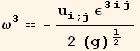
![]()
![]()
In this expression, ![]() is the average rotation of a deformable volume element in the plane {1,2}.
is the average rotation of a deformable volume element in the plane {1,2}.
Compatibility conditions
There are three displacements ![]() , but six different strain components
, but six different strain components ![]() . In fact if we calculate the second derivatives of
. In fact if we calculate the second derivatives of ![]() , and there combination
, and there combination
![]()
![res = res0/.{CovariantD[ℰdd[red @ i, red @ j], {l1_, l2_}] :>CovariantD[(1/2 (CovariantD[ud[red @ i], red @ j] + CovariantD[ud[red @ j], red @ i])), {l1, l2}]}](HTMLFiles/index_48.gif)
![]()
![]()
we find other conditions to which the ![]() are subjected. In flat space,
are subjected. In flat space, ![]() is symmetrical with respect to its covariant derivatives, so that we verify that it gives zero,
is symmetrical with respect to its covariant derivatives, so that we verify that it gives zero,

![]()
![]()
The compatibility conditions are then :
![(*6.4*)ResultFrame[res64 = CovariantD[ℰdd[red @ i, red @ j], {red @ k, red @ l}] euuu[red @ i, red @ k, red @ m] euuu[red @ j, red @ l, red @ n] == 0]](HTMLFiles/index_56.gif)
![]()
The above matrix {m,n} is symmetrical and the six equations corresponding to {m,n}={1,1},{2,2},{3,3},{1,2},{2,3},{3,1} give zero.
![]()
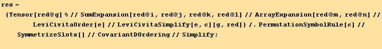
![restable = {res[[1, 1]] == 0, res[[2, 2]] == 0, res[[3, 3]] == 0, res[[1, 2]] == 0, res[[2, 3]] == 0, res[[3, 1]] == 0}//TableForm](HTMLFiles/index_60.gif)
![]()
In cartesian coordinates the compatibility equations are (the covariant derivatives being then identical to partial derivatives):
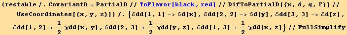
In the covariant form we would have written :

Condition of Equilibrium and Equation of Motion
Figure 6.2
![[Graphics:HTMLFiles/index_82.gif]](HTMLFiles/index_82.gif)
Figure 6.2 Stress acting on a volume element.
The edges of the infinitesimal block of material (figure), are the vectors,
![]()
![]()
The face on the right hand side is ![]() equal to,
equal to,
![]()
![]()
![]()
The difference between the forces applied on opposite faces are then given by,
![]()
![]()
![]()
![]()
![]()
![]()
Similar expression are obtained for the two others opposite faces, and globally we have
![]()
![]()
![]()
![]()
![]()
![]()
This expression is identical to (see also the section treating the Gauss theorem in three dimensions, for a similar result)
![]()
![]()
and,
![]()
![]()
In addition, we see that ![]()
![]()
![]()
![]() is the volume dV of the block, so that the resultant of all the stresses is
is the volume dV of the block, so that the resultant of all the stresses is
![]()
![]()
Superposed to the stress we can have an external force
![]()
![]()
The system is in equilibrium if
![]()
![]()
Condition of Equilibrium :
![(*6.5*)ResultFrame[res65 = (TotalForce = res[[1, 2]]) == 0]](HTMLFiles/index_115.gif)
![]()
The equilibrium of the moments is itself satisfied by the symmetry of the stress tensor (as shown in the above section on the stress tensor).
Dynamic equation
In the limit of small motion the Lagrangian or particle formulation and the Eulerian or field formulation coincide. We can associate a certain time dependent velocity to each particle, but since the particle always stay close to the position it has at rest, the same velocity is also associated with that point in space.
We define the usual notations,
![]()
![]()
![]()
![]()
If ρ is the mass density, we have the dynamic equation,
![(*6.6*)ResultFrame[res66 = TotalForce[[1]] == (totalforce = ρ Tensor[OverDot[u, 2], {red @ i}, {Void}] - TotalForce[[2]]) ]](HTMLFiles/index_121.gif)
![]()
Fundamental Equations of the theory of Elasticity
We have the basic equations describing the equilibrium and the small motions of an elastic solid :
(1) the kinematic relation ![]() ==
==![]() (
(![]() +
+![]() )
)
(2) the equilibrium condition ![]() +
+ ![]() ==0 or the dynamic equation
==0 or the dynamic equation ![]() ==ρ
==ρ ![]() -
-![]()
(3) the Hooke's laws ![]() =
= ![]()
![]()
and ![]() ==
== or
or ![]() ==2 μ
==2 μ ![]() +λ
+λ ![]()
![]()
They form 6+3+6 = 15 component equations, which contain 15 unknowns (6 ![]() , 6
, 6 ![]() , and 3
, and 3 ![]() ) .
) .
We recall first here the Hooke's laws (equations (4.3) and (4.11)):
![]()

If the material is anisotropic, we have from (2) and (3) in the cell grey box,
![res = (CovariantD[(σ§uu[i, j]//ToFlavor[red, black])/.ℰdd[red @ i_, red @ j_] →ℰ§dd[red @ i, red @ j], red @ j]//FullSimplify) == totalforce](HTMLFiles/index_146.gif)
![]()
If the material is anisotropic but homogeneous, the covariant derivative of the elastic modulus vanishes,
![(*6.7*)ResultFrame[res67 = (res/.CovariantD[uuuu[i_, j_, k_, l_], m_] →0)//Simplify]](HTMLFiles/index_148.gif)
![]()
If the material is isotropic, we have (we first calculate ![]() as a function of the displacements),
as a function of the displacements),
![]()
![]()
![]()
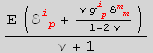
Introducing the dynamic equation ![]() ==ρ
==ρ ![]() -
-![]() == totalforce :
== totalforce :
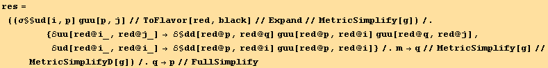
![res = (CovariantD[res1[[2]], red @ j]//CovariantDSimplify[, g, e]//MetricSimplifyD[g]//SymmetricStandardOrder[u, {2, 3}])/.p→j//Simplify ; (*6.8*)](HTMLFiles/index_158.gif)
![]()
This fundamental equation can also be expressed using Lame moduli (equation (4.7)),
![]()
![(*6.9*)ResultFrame[res69 = (res68/.LameRule//Simplify) ]](HTMLFiles/index_162.gif)
![]()
Taking the divergence of the above equation,
![]()
![]()
![]()
![]()
![]()
We can then introduce the Laplace operator notation Δ and write using the preceding identification,
so that the preceding equation is simply in absence of external force,
![]()
![]()
![]()
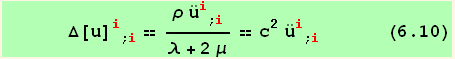
where c has the dimension of a velocity.
A second important equation is obtained when taking the curl of equation (6.9) :
![]()
![]()
![]()
![]()
The term ![]() in the parenthesis, symmetrical, together with
in the parenthesis, symmetrical, together with ![]() gives zero, after summation on k and l,
gives zero, after summation on k and l,
![]()
![]()
![]()
![]()
An up-down swap of the indices gives an equivalent expression
![]()
![]()
When there is no force in equ. (6.11)
![]()
![]()
![]()
with
![]()
1) Any solution of equ. (6.9) without external force, must satisfy equ. (6.10) and (6.11).
Equation (6.13) has a trivial solution ![]()
![]() = 0, or curl [u] = 0.
= 0, or curl [u] = 0.
A vector field which satisfies this condition derives from a potential φ, the displacement potential.
![]()
![]()
![]()
![]()
![]()
If we introduce this result in (6.9) when ![]() = 0, and take into account the relation
= 0, and take into account the relation ![]() ==
==![]() .
.
![]()
![((%[[1, 1]] + (%[[1, 2]]/.u_a_^a_^(; b_) :→u_b^b^(; a)) - %[[2]])/(λ + 2 μ)/.ρ-> (λ + 2 μ) c^2//Simplify) == 0 ; (*6.14*)](HTMLFiles/index_200.gif)
![]()
![]()
2) On the other hand, a solution of equ. (6.10) has a trivial solution ![]() = 0, or div [u] = 0. Carried into (6.9) gives
= 0, or div [u] = 0. Carried into (6.9) gives
![]()
![]()
![]()
The general solutions of both equations (6.14) and (6.15) is in cartesian coordinates (![]() ==
==![]() ),
),
![]()
![]()
with three arbitrary functions ![]() . This represents an elastic wave propagating with the velocity c (or
. This represents an elastic wave propagating with the velocity c (or ![]() in the case of eq.(6.14)). The solutions with curl [u] = 0 are dilatational waves, while those with div [u] = 0 are shear waves.
in the case of eq.(6.14)). The solutions with curl [u] = 0 are dilatational waves, while those with div [u] = 0 are shear waves.
We define first the operation TotalTimeDerivation[labs, i][T, t] which is the sum of the partial derivative of a tensor T with respect to time t, and of the spatial coordinates in the parameter defined by the labels labs (see the equation for p and a below).
![]()
We adopt here the Eulerian formulation : coordinate system tied to the fluid, so that a particle of the fluid has a fixed position ![]() . In the lab frame, this position is
. In the lab frame, this position is ![]() and depends generally on time. Its velocity
and depends generally on time. Its velocity ![]() is given by,
is given by,
![]()
![]()
and any field quantity p is
![]()
![]()
![]()
Note : here we cannot use PartialSum, because time t do not belong to the base indices (it is not relativistic!).
The acceleration is,
![]()
![]()
![]()
![]()
with the components,
![(*6.16*)ResultFrame[res616 = au[red @ i] == PartialD[vu[red @ i], t] + vu[red @ j] CovariantD[vu[red @ i], red @ j]]](HTMLFiles/index_226.gif)
![]()
where we have used the fact that,

![]()
Result (6.15) contains two terms, ![]() represents the change of velocity when the flow is non stationary, while
represents the change of velocity when the flow is non stationary, while ![]()
![]() represents the change of velocity when the flow moves during dt to another point where the velocity is different.
represents the change of velocity when the flow moves during dt to another point where the velocity is different.
Dynamic equation of the fluid flow :
We use result (6.5) derived for solids, but now ![]() is the acceleration
is the acceleration ![]() of the particles of fluid
of the particles of fluid
![]()
![]()
![]()
![]()
![]()
On the other hand, time derivative of the kinematic relation (6.2) ![]() ==
==![]() (
(![]() +
+![]() ) gives,
) gives,
![]()
![]()
It is interesting here to split this equation into a rate of dilatation e and a rate of distortion .
In chapter 4, we have defined the parameters e and s, and we introduce,
![]()
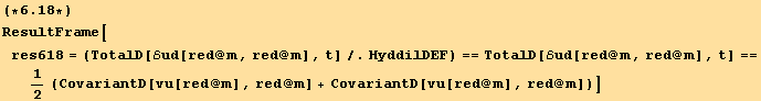
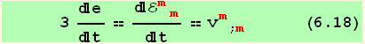
We define,
![]()
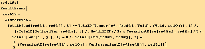
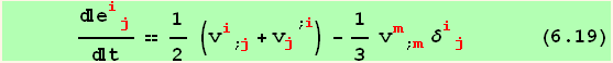
If the fluid is incompressible, ![]() =0 , or
=0 , or ![]() = 0, so that in this case equ. (6.18) becomes,
= 0, so that in this case equ. (6.18) becomes,
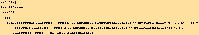
![(*6.2*)ResultFrame[res620 = distortion[[1]] == (distortion[[2]]/.{CovariantD[vu[red @ m], red @ m] →0}) == TotalD[ℰud[red @ i, red @ j], t]]](HTMLFiles/index_254.gif)
and there is no difference between ![]() and
and ![]() .
.
In a fluid at rest, or also in an inviscid fluid in motion, the pressure is isotropic, while in a viscous fluid in motion, the volume elements are undergoing a deformation and the compressible stresses have different magnitude in different directions. If we still want to define a pressure in the fluid, it can be the average of normal stress, counted positive when compressive. From the rule HyddilDEF which defines the hydrostatic stress s and the cubic dilation e, we have :
![]()
![]()
Introducing the above relation in ![]() given in chapter 4
given in chapter 4
![]()
we have,
![]()
![]()
Finally, when we introduce the constitutive equation (4.16) ![]() ==2 μ
==2 μ ![]() ,
,
![]()
![]()
![]()
The elimination of ![]() between equation (6.21) and equation (6.17) leads to the important Navier-Stokes equation for the kinetic evolution of a viscous fluid in presence of external forces :
between equation (6.21) and equation (6.17) leads to the important Navier-Stokes equation for the kinetic evolution of a viscous fluid in presence of external forces :
First we note that we consider an incompressible fluid, ![]() =0 , or
=0 , or ![]() = 0, so that :
= 0, so that :
![]()
![]()
![]()

![]()
![]()
![]()
![]()
This equation, which contains four unknown, ![]() and p, together with the continuity equation
and p, together with the continuity equation ![]() = 0, determines the flow of the fluid.
= 0, determines the flow of the fluid.
Streamlines
The streamlines of the velocity field ![]() are the lines everywhere tangent to the vector v. The streamlines passing through all the points of a closed curve C, form a tube called a stream tube.
are the lines everywhere tangent to the vector v. The streamlines passing through all the points of a closed curve C, form a tube called a stream tube.
Let us choose a coordinate system ![]() such that,
such that,
![]()
![]()
![]()
![]()
![]()
where the considered curve C is the quadrilateral defined by {dr, ds}. Its area is,
![]()
![]()
and the flux of fluid through C is,
![]()
![]()
If we consider another cross section ![]() = const, of the stream tube, this cross section is again dA. Along the steamlines,
= const, of the stream tube, this cross section is again dA. Along the steamlines, ![]() and
and ![]() do not vary, and
do not vary, and
![]()
![]()
Due to the continuity equation ![]() = 0, this is zero. The same amount of fluid passes through all the cross sections of a stream tube. It is interesting to notice that this result valid in the obvious case of an incompressible fluid, needs only the condition
= 0, this is zero. The same amount of fluid passes through all the cross sections of a stream tube. It is interesting to notice that this result valid in the obvious case of an incompressible fluid, needs only the condition ![]() = div v = 0, to be valid. We will see later a case of application which is not obvious.
= div v = 0, to be valid. We will see later a case of application which is not obvious.
If the fluid flow is stationary, ![]() = 0, the streamlines are the paths followed by fluid particles during their motion in the flow field. If the flow is not stationary, the shape of the streamlines changes with time. The pathlines
= 0, the streamlines are the paths followed by fluid particles during their motion in the flow field. If the flow is not stationary, the shape of the streamlines changes with time. The pathlines ![]() = const, are then different fromthe streamlines.
= const, are then different fromthe streamlines.
When the fluid is at rest, all the velocity terms cancel in the Navier-Stokes equation. This determines the hydrostatic pressure,
![]()
![]()
![]()
![]()
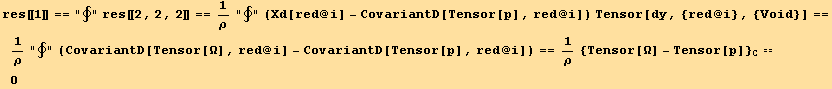
Since p is a scalar, ![]() must be a gradient field, and its curl is zero, otherwise, the fluid cannot be in equilibrium.
must be a gradient field, and its curl is zero, otherwise, the fluid cannot be in equilibrium.
![Xd[red @ i] == CovariantD[Tensor[Ω], red @ i] curl X == 0 or TCurl[, g, red/@{i, j, k}, e][Xd[red @ i] u[red @ i]][[Range[1, 2]]] == 0](HTMLFiles/index_308.gif)
![]()
When the viscosity is negligeable (like in water or air), the Navier-Stokes equation reads,
![]()
![]()
![]()
or from (6.16) ![]() ==
==![]()
![]() +
+![]() ==
== ![]() , and lowering the indices,
, and lowering the indices,
![]()

Circulation integral of the velocity on a closed curve, vorticity
![]()
![]()
![]()
![]()

![]()
Only the second term in the integration remains, so that we have using equ. (6.23)
![]()
Finally, we see that for an inviscid fluid moving in a conservative force field,
![]()
![]()
for any closed curve moving with the particles of fluid. In particular, this is true for an infinitesimal curve bounding an area dA. From Stokes theorem, (equ.5.8), we deduce that,
![]()
![]()
![]()
![]()
![]()
![]()
![]()
![]()
Similarly to the velocity field and streamlines of the flow, we can define the vorticity field and the vorticity lines or vortex filaments.
The product ω.dA is the flux of vorticity through the cross section dA of a vortex tube passing through all the points of the perimeter C of dA. This flux is constant.
Unsteady flows frequently start at rest; steady flows frequently approach from infinity with a uniform velocity toward an obstacle. In both case curl(v) = 0, and from equ.(6.26) valid for any area, curl(v) remains throughout zero : the flow field is a gradient field
![(*6.27*)ResultFrame[res627 = vd[red @ i] == CovariantD[Tensor[Φ], red @ i]]](HTMLFiles/index_339.gif)
![]()
This kind of velocity field is called a potential flow. Using the continuity equation ![]() = 0 leads to
= 0 leads to
![]()
![]()
Introducing (6.27) into (6.22) gives
![res = (res622/.μ→0/.vu[i_] :→ContravariantD[Tensor[Φ], i]/.Tensor[Overscript[v, .], {red @ i}, {Void}] :→ContravariantD[Tensor[Overscript[Φ, .]], red @ i]) == 0](HTMLFiles/index_344.gif)
![]()
or equivalently :
![]()
![]()
so that ![]() being symmetrical
being symmetrical ![]() =
= ![]() ,
,
![]()
![]()
![]()
![]()
![]()
![]()
![]()
![]()
which gives an equation for the pressure p
![]()
![p_ (; i) == -ρ (1/2 Φ^(; j) Φ_ (; j) + Overscript[Φ, .]) _ (; i) + X_i^i (6.28)](HTMLFiles/index_360.gif)
The boundary condition for (6.28) concerns the velocity component normal to the boundary S of the domain of the fluid flow. If ![]() is the unit normal to S, the normal component of v is
is the unit normal to S, the normal component of v is
![]()
![]()
This is subject to an integrability condition by the divergence theorem, equ.(5.7) so that ![]()
![]() must be chosen such that,
must be chosen such that,
![(*6.29*)ResultFrame[res629 = ∫ vu[red @ i] dAd[red @ i] == 0] \S](HTMLFiles/index_366.gif)
![]()
This section is concerned by the seepage flow through a porous medium. It is a randomly multiconnected medium whose channels are randomly obstructed. The quantity that measures how "holed" the medium is due to the presence of these channels is called the porosity of the medium. Another important quantity, analogous to the conductivity of a network of resistors, is the Darcy permeability: it decreases continuously as the porosity decreases, until a critical porosity reached when it vanishes. Close to this critical porosity, the regime is fractal (see Physics and Fractal Structures, Jean-François Gouyet, Springer-Verlag, Berlin, New York, and Masson, 1996), and the seepage flow is described by the model of invasion percolation. All the present studies are supposed to take place far from the critical region, so that the mean-field approaches remain valid.
The flow in the channels are mostly dominated by viscous friction, and its velocity is proportional to the pressure gradient.
Let ![]() be the force acting on a unit of the fluid volume, and v the mean velocity (filter velocity) of the fluid flow with respect to an infinitesimal bulk cross section. To make the fluid move,
be the force acting on a unit of the fluid volume, and v the mean velocity (filter velocity) of the fluid flow with respect to an infinitesimal bulk cross section. To make the fluid move, ![]() -
-![]() must be different from zero. If the pore geometry has no preferential direction, v follow the direction of the force field
must be different from zero. If the pore geometry has no preferential direction, v follow the direction of the force field ![]() -
-![]() .
.
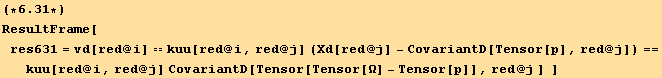
Darcy's law
![(*6.3*)ResultFrame[res630 = vd[red @ i] == k (Xd[red @ i] - CovariantD[Tensor[p], red @ i]) == k CovariantD[Tensor[Tensor[Ω] - Tensor[p]], red @ i] ]](HTMLFiles/index_373.gif)
![]()
Some porous media are anisotropic (linear channels, layers,...) and the Darcy's law takes the more general expression
![]()
and the velocity field satisfies the continuity equation,
![ := vu[red @ i] d[red @ i] (*6.32*)](HTMLFiles/index_377.gif)
![]()
![]()
Combining this condition with equ.(6.31) gives,
![]()
![]()
But in an homogeneous medium, the Darcy coefficient do not vary in space and ![]() =0.
=0.
![]()
![]()
and finally in the isotropic case,
![]()
![]()
![]()
![]()
This gives the Poisson equation,
![]()
![]()
or in absence of local force, the Laplace equation,
![]()
![]()
Flügge discusses here the fact that ![]() is always found symmetric on practical examples, but emphasizes that there is a lack of convincing general proof.
is always found symmetric on practical examples, but emphasizes that there is a lack of convincing general proof.
We will admit the symmetry of k.
![]()
![]()
Action of the fluid moving in a porous medium, on the solid matrix.
![[Graphics:HTMLFiles/index_396.gif]](HTMLFiles/index_396.gif)
Figure 6.4 Volume element of a porous medium
The volume in the above figure is supposed infinitesimal, but its dimension must be much larger than the size of the pores. This allows, far from the critical porosity, to make an effective field approximation. The surface of pores in the section {ds, dt} is φ || ds×dt ||. From equation (4.1), the force due to the the stress acting on the cross section {ds, dt} is,
![]()
![]()
the force due to the fluid pressure and acting on the cross section φ ![]()
![]() is,
is,
![]()
![]()
so that the total force acting on the face {ds, dt} is,
![]()
![]()
Replacing the TotalForce in equation (6.5) by the above force components we have (we define σ§ji = ![]() -
-![]()
![]()
![]() ),
),
![]()
![]()
![]()
![]()
![]()
Note this equation shows that a constant pressure produces a stress if the porosity φ is variable.
To study a stress problem in presence of seepage flow, we have to consider the three equations, (4.11), (6.2), and (6.37).
![]()
| Created by Mathematica (November 27, 2007) |