9. Theory of Shells
Initialization
![]()
![]()
![]()
![]()
![]()
![]()
![]()
![]()
![]()
![]()
![]()
![]()
![]()
![]()
![]()
![]()
![]()
![]()
Notation of the 2d and 3d litteral indices :
Latin characters are used for 3d, greek characters are use for 2d spaces.
Then SymbolSpaceDimension[index] gives the dimension of the space concerned by index.
SymbolSpaceDimension[Symbol] gives the
![]()
![]()
![]()
![]()
![]()
![]()
![Print[General surface (z≠0)]](HTMLFiles/index_25.gif)
![]()
![Print[Middle surface (z = 0)]](HTMLFiles/index_27.gif)

![]()
| e | basis symbol |
| g | metric tensor |
| permutation tensor | |
| Christoffel symbol | |
| η | strain tensor |
| basis deformed symbol |
![]()
| a | basis symbol |
| a | metric tensor |
| e | permutation tensor |
| Γ | Christoffel symbol |
| E | strain tensor |
| basis deformed symbol | |
| deformed metric tensor | |
| curvature deformed tensor |
![]()
![]()
![]()
![]()
![]()
![]()
Shell Geometry
A point B on a shell of uniform thickness h, is defined by its coordinates {![]() ,
,![]() }. The coordinate
}. The coordinate ![]() =z normal to the surface is counted from its middle, so that the outer faces are at z = ±h/2. We want to express following the preceding chapter, all the quantities associated with the point B like
=z normal to the surface is counted from its middle, so that the outer faces are at z = ±h/2. We want to express following the preceding chapter, all the quantities associated with the point B like ![]() ,
,![]() ,
,![]() , etc..., in terms of the corresponding quantities
, etc..., in terms of the corresponding quantities ![]() ,
,![]() ,
,![]() associated with the midsurface point A [
associated with the midsurface point A [![]() ,0] (figure below). The points C and D have the same coordinates
,0] (figure below). The points C and D have the same coordinates ![]() +
+![]() , so that the vectors AC and BD in the planes have the same components
, so that the vectors AC and BD in the planes have the same components ![]() but not the same
but not the same ![]() and
and ![]() .
.
![[Graphics:HTMLFiles/index_58.gif]](HTMLFiles/index_58.gif)
Figure 9.1 Section through a shell.
Starting from
![]()
![]()
![]()
![]()
differentiating with respect to α,
![]()
![]()
and using (8.12)
![]()
![]()
with,
![]()
![]()
We have defined the tensor ![]() which relates the base vectors at points A and B. To obtain a similar relation between the contravariant quantities, we try,
which relates the base vectors at points A and B. To obtain a similar relation between the contravariant quantities, we try,
![]()
![]()
Then,
![]()
![]()
![]()
![]()
![]()
![]()
which allows to calculate the ![]() . As they are fractions of a polynomial in z we expand
. As they are fractions of a polynomial in z we expand ![]() as a power expansion in z up to quadratic terms :
as a power expansion in z up to quadratic terms :
![]()
![]()
![]()
![]()
![]()
![]()
![]()
![]()
![]()
![]()
![r3[red @ β_, red @ α_] = rul[red @ β, red @ α][[3]]/.r2[red @ β, red @ ρ] ; (*9.5*)](HTMLFiles/index_90.gif)

![]()
Now, from the definition of the metric tensor,
![]()
![]()
and also,

![]()
![]()
Other formula involving the important tensors ![]() and
and ![]() will be needed in the following :
will be needed in the following :
By differentiation of (9.4)
![]()
![]()
![]()
![]()
![]()
![]()
Note that the 3d metric g tensor is correctly used here, as its submatrice in the 2d space is identical to the metric tensor a.
We can expand ![]() , and use the symmetry (8.24) (Gauss-Codazzi's relations) and (9.2) to write,
, and use the symmetry (8.24) (Gauss-Codazzi's relations) and (9.2) to write,
We shall also need the determinant of ![]() :
:
![]()
![]()
![]()
![]()
Explicitely, using equ.(9.2) :
![]()
![]()
![]()
![]()
![]()
![]()
Or introducing the Gaussian curvature b and the mean curvature ![]() :
:
![]()
![]()
![]()
![]()

![]()
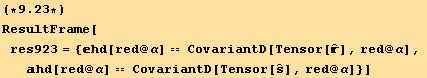
![(*9.13*)ResultFrame[res913 = ((res[[1]]//FullLeviCivitaExpand[e, a])/.{adu[δ_, δ_] →NDim}) == res[[2]]]](HTMLFiles/index_129.gif)
![]()
![]()
![]()
![]()
![]()
Now, from (9.4) and (9.11)
![]()
![]()
![]()
![]()
![]()
![]()
Together with (9.13) gives :
![]()
![(res914/.{%[[2]] →%[[1]]}//FullLeviCivitaExpand[e, g])/.{gdu[δ_, δ_] →NDim} (*9.16*)](HTMLFiles/index_142.gif)
![]()
![]()
![]()
![]()
while for the derivative of the determinant μ with respect to the coordinate normal to the midsurface. Starting from (9.13) :
![]()
![]()
and using (9.14) and (9.2)
![]()
![]()
![]()
![]()
In Tensorial 4, derivation with respect to a particular coordinate is not expanded (so we use /.{red@3→red@z}/.{red@z→red@3} to allow it).
![]()
![]()
![]()
![]()
![]()
![]()
![]()

![]()
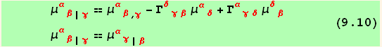
Expressions for the Christoffel symbols ![]() and
and ![]() , and the "permutation tensor"
, and the "permutation tensor" ![]() and
and ![]() at point B of the above figure.
at point B of the above figure.
We use the expressions of chapter 5, for the Christoffel symbols, together with (9.1) and (9.3):
![]()
![]()
![]()
![]()
![]()
![]()
![]()
![]()
![]()
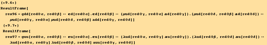
Then, with (9.10) and (9.4)
![]()
![]()
![]()
![]()
![]()
![(*9.18*)ResultFrame[res918 = res1[[1]] == res1[[2]] + zero/.res3[[2]] →res3[[1]]//MetricSimplify[g]//SymmetrizeSlots[]//TensorSimplify]](HTMLFiles/index_180.gif)
![]()
Similarly, we obtain (don't forget that ![]() is zero because
is zero because ![]() is on the surface : we must add "False" in EvaluateDotProducts) ,
is on the surface : we must add "False" in EvaluateDotProducts) ,
![]()

![]()
![]()
and with (8.11) and (8.12)

![]()
![]()
![]()
![]()
Then, with (8.9), (9.3) and ![]() =
=![]() on z = 0,
on z = 0,
![]()
![(res = PartialD[d[red @ 3], red @ β] . u[red @ α]) == (res1 = (res//ChristoffeluSymbol[, Γb, ρ]//EvaluateDotProducts[, g])) <br />(*9.2*)](HTMLFiles/index_196.gif)
![]()
![]()
![]()
![]()
Introduction of the permutation tensor
![]()
![]()
![]()
![]()
![]()
![]()
![]()
![]()
Now we use (9.4),
![]()
![(Times[μud[red @ δ, red @ α], #] &/@res )/.%/.{γ→δ, δ→γ}//MetricSimplify[g]//LeviCivitaOrder[e]//LeviCivitaOrder[eb] (*9.21*)](HTMLFiles/index_210.gif)
![]()
![]()
![]()
![]()
together with (9.12)
![(*9.22*)ResultFrame[res922 = res921[[2]] == res921[[1]]/.res912[[2]] →res912[[1]]]](HTMLFiles/index_215.gif)
![]()
Kinematics of Deformation
After a deformation of the shell, a generic point at position r like B is transformed into ![]() (figure below)
(figure below)
![]()
![]()
and for the corresponding point A on the middle surface,
![]()
![]()
The same coordinates are associated to each material point before and after deformation, but the corresponding basis vectors are deformed with the body, and we have,
![]()
![[Graphics:HTMLFiles/index_224.gif]](HTMLFiles/index_224.gif)
Figure 9.2 Section through a shell before and after deformation.
Hypothesis : during the deformation, the normals are conserved. This means that after deformation, all the points which were on a normal to a point of the middle surface beforev deformation all remain on the same normal. This leads to assume that,
![]()
![]()
Equation (6.2) gives the relation between strain and displacement (with the notations corresponding to the middle surface),
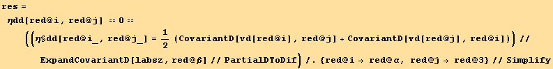
![(*9.24*)ResultFrame[res924 = ηdd[red @ i, red @ j] == (η§dd[red @ i_, red @ j_] = 1/2 (CovariantD[vd[red @ i], red @ j] + CovariantD[vd[red @ j], red @ i])) ]](HTMLFiles/index_227.gif)
![]()
When we take i = α and j = 3, we have
![]()
so that the conservation of normals gives,
![(*9.25*)ResultFrame[res925 = (res[[3, 2]]//SymmetricStandardOrder[Γb]) == 0//Simplify]](HTMLFiles/index_231.gif)
![]()
Another reasonable hypothesis is to consider that the length of the normal (shell thickness) does not vary. This is because the shell is thin and there is no stress ![]() along the direction
along the direction ![]()
![]()
![]()
Note that the shell is not in a state of plain strain, but rather of plain stress which includes the stress coming from the bending: the statement ![]() = 0, must not be inserted in Hooke's law.
= 0, must not be inserted in Hooke's law.
From (9.25) applied to the middle surface, using (8.13) allows to introduce the curvature tensor,

![]()
Now we need to get ![]() , the normal vector to the deformed shell element. From
, the normal vector to the deformed shell element. From ![]() ==r+v, differentiated with respect to
==r+v, differentiated with respect to ![]() , taking z = 0, and writing
, taking z = 0, and writing ![]() = lim
= lim ![]()
![]()
![]()
and with (8.22),
![]()
![]()
but (see figure 9.2) ![]() = w does not depend on
= w does not depend on ![]() so that
so that ![]() = 0, and
= 0, and
![]()
![]()
![]()
![]()
![]()
An alternate form can be derived using (9.26)
![]()
![]()
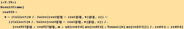
![(*9.27*)ResultFrame[res927 = res2[[1]] == (res2[[2]]/.res926[[1, 2]] → res926[[2]] - res926[[1, 1]]//TensorSimplify//Simplify)]](HTMLFiles/index_259.gif)
![]()
![]() and
and ![]() being unit vectors,
being unit vectors, ![]() —
— ![]() is the angle of rotation of the normal. It is a plane vector (decomposition on
is the angle of rotation of the normal. It is a plane vector (decomposition on ![]() ), and
), and ![]() are the components of a vector ω
are the components of a vector ω
![]()
![]()
![]()
![]()
Note also that ![]() ==
==![]()
![]()
Considering figure (9_2), we see that,
![]()
![]()
and,
![]()
![]()
so that,
![]()
On the other hand we have,
![]()
![]()
![]()
![]()
![]()
![]()
![]()
which, with (9.2) and (9.8), is equivalent to,
![]()
![{(res98/.{β→δ})[[1]] → (res98/.{β→δ})[[2]] } <br /><br />(*9.31*)](HTMLFiles/index_290.gif)
![]()
![]()
![]()
![]()
We want now to calculate the stress ![]() (from (9.24))
(from (9.24))
![]()
![]()
![]()
![]()

![]()
Using now (9.18) and (9.19)
![]()
![]()
![]()
![]()
![]()
Now we use the relation (9.31) to replace the ![]() on the right hand side :
on the right hand side :

This expression simplifies after introduction of relation (9.4)
![]()
![]()
![]()
![]()
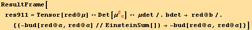
By interchanging α and β we obtain ![]()

Strain of the middle surface E
We have made the basic assumption that the normals are conserved, so that the deformation of a shell element depends only on the deformation of the middle surface. It is then possible to express ![]() in terms of the strain of the middle surface and of its change of curvature. The strain of the middle surface E, then corresponds to setting z = 0 in (9.33). When z = 0, the various
in terms of the strain of the middle surface and of its change of curvature. The strain of the middle surface E, then corresponds to setting z = 0 in (9.33). When z = 0, the various ![]() become delta functions (see equ.(9.2)).
become delta functions (see equ.(9.2)).
![(*9.34*)ResultFrame[res934 = res933/.{η→ℰ, z→0}//CovariantDSimplify[μ]//MetricSimplifyD[μ]//SymmetricStandardOrder[b] ]](HTMLFiles/index_319.gif)
![]()
The quantities a, ah, b, ![]() , w, η, E are symmetrical with respect to their indices.
, w, η, E are symmetrical with respect to their indices. ![]() below is not.
below is not.
Metric tensor for the deformed middle surface :
From equations (2.1) and the relation ![]() =
= ![]() /2, and using the present notations, we can define the metric tensor for the deformed middle surface by,
/2, and using the present notations, we can define the metric tensor for the deformed middle surface by,
![]()
![]()
Curvature tensor for the deformed middle surface :
Note : As the head of ![]() is not a Symbol, we have used the symbol bh as an alias in the Inputs (via TensorLabelFormat[bh,OverHat[b]]) .
is not a Symbol, we have used the symbol bh as an alias in the Inputs (via TensorLabelFormat[bh,OverHat[b]]) .
We shall consider the curvature change ![]() ==-
==-![]() +
+![]() because in this case the metric tensor is independent on the deformation.
because in this case the metric tensor is independent on the deformation.
![]()
Then we have, using Flügge's notation,
![]()
![]()
![]()
![]()
![]()
![]()
![]()
![]()
and if we neglect a term quadratic in the strain, we may write,
![]()
![]()
This expression shows that ![]() ≠
≠ ![]() -
- ![]() .
.
We need to calculate now ![]() . From equ. (8.9) applied to the deformed middle surface,
. From equ. (8.9) applied to the deformed middle surface,

![]()
![]()
and if we differentiate (9.27) and use (8.23) we can explicit ![]()
![]()
![]()
![]()
![]()
so that when v becomes ![]() (we replace here a symbol v by a tensor
(we replace here a symbol v by a tensor ![]() , so that we will need to apply UnnestTensor to expand the left hand side):
, so that we will need to apply UnnestTensor to expand the left hand side):
![]()
![]()
![]()
![]()
![]()
![]()
Remember that ![]() is intentionally not expanded
is intentionally not expanded
We can expand this term using :
![]()
![]()
Deformed base vector ![]()
From its definition, together with equation (8.19),
res819 = PartialD[Tensor[u],red[β]]==(bud[red[γ],red[β]]ud[red[γ]]+PartialD[ud[red[3]],red[β]])au[red[3]]+au[red[α]](-bdd[red[β],red[α]]ud[red[3]]+PartialD[ud[red[α]],red[β]]-ud[red[γ]]Γudd[red[γ],red[β],red[α]])
![]()
![]()
![]()
![%/.(CovariantD[ud[red @ α], red @ β]//ExpandCovariantD[labs0, red @ γ]//PartialDToDif) → CovariantD2d[ud[red @ α], red @ β] ;](HTMLFiles/index_370.gif)
![]()
![]()
![]()
Using the replacements of ![]() and of
and of ![]() (via resâ3 and resâ3β above), the cancellation of the covariant derivatives of basis vectors,
(via resâ3 and resâ3β above), the cancellation of the covariant derivatives of basis vectors,
and equ. (8.9) ![]() →-
→-![]()
![]() ,
,
![]()
![]()
![rul89 = {PartialD[Tensor[, {Void}, {red[3]}], red[α_]] → -Tensor[b, {Void, Void}, {red[α], red[ρ]}] Tensor[, {red[ρ]}, {Void}]}](HTMLFiles/index_381.gif)
![]()
![]()
![]()
![]()
![]()
![]()
![]()
in which we only conserve linear terms in the displacements
![]()
![]()
![]()
![]()
![]()
![]()
![]()
![]()
![]()
![]()
![]()
![]()
![]()
![]()
From (9.37) we deduce now ![]()
![]()
![]()
We can expand equation (9.39) use (9.28) and replace ![]() by its expression (9.34)
by its expression (9.34)
![]()
![]()
![]()
![]()
![]()
![]()
Note that due to the Codazzi equation (8.24) ( ![]() ==
==![]() and
and ![]() ==
==![]() ) to property (9.28) and the dummy index in
) to property (9.28) and the dummy index in ![]()
![]() , the indices α and β can be interchanged in the first, third, and the fifth terms. This is not the case for the second and fourth terms, so that
, the indices α and β can be interchanged in the first, third, and the fifth terms. This is not the case for the second and fourth terms, so that ![]() ≠
≠ ![]() .
.
Our purpose now is to express ![]() in terms of
in terms of ![]() and
and ![]()


We expect that the rhs contains a factor z ![]() .
.
The fourth term (resA) already contains a factor z :

![]()
For the other terms we make use of equation (9.2),
![]()
![]()
so that, the terms containing ![]() gives :
gives :
![]()
![]()
![]()
![]()
We shall also need the following identity (an invariance by permutation of b and μ) :
![]()
![]()
![]()
we find another term with a factor z :
![]()
We call res4 the term which does not contains the factor z,
![]()
![]()
First we consider the coefficient of w,
![]()
![]()
![]()
![]()
![]()
![]()
Remains finally the following term in res4 to consider :
![]()
![]()
![]()
![]()
![]()
Here we use equation (9.41):
![]()
![]()
![]()

![]()
![]()
![]()
We recognize in this expression the factor :
![]()
![]()
![]()
Therefore, we can write :
![]()
![]()
![]()
![]()
`` This equation shows that the strain ![]() and hence the stress
and hence the stress ![]() only depends on the deformation of the middle surface and that our kinematic relations, in particular (9.33), will yield zero strain when the shell is subjected to a rigid body displacement ″
only depends on the deformation of the middle surface and that our kinematic relations, in particular (9.33), will yield zero strain when the shell is subjected to a rigid body displacement ″
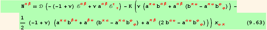
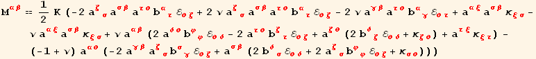
Stress Resultants and Equilibrium
Stress Resultants and Equilibrium
In a shell the stress systems of plates and slabs are combined. There is a membrane force tensor ![]() corresponding to the tension-and-shear of the plane slab and a moment tensor
corresponding to the tension-and-shear of the plane slab and a moment tensor ![]() , whose components are bending and twisting moments, and, as in a plate, it is inseparable from transverse shear forces
, whose components are bending and twisting moments, and, as in a plate, it is inseparable from transverse shear forces ![]() . Due to the curvature of the shell element, all these forces and moments, which contribute to the equilibrium of the shell element, interfere.
. Due to the curvature of the shell element, all these forces and moments, which contribute to the equilibrium of the shell element, interfere.
![[Graphics:HTMLFiles/index_476.gif]](HTMLFiles/index_476.gif)
Figure 9.3 Section through a shell.
In this figure, we have selected an arbitrary line element ds==![]()
![]() on the middle surface. The set of normals to this line element ds generates a section element of thickness h. Due to the curvature and twist of the surface, these normals are not really parallel, and even not in the same plane. This must be taken into account.
on the middle surface. The set of normals to this line element ds generates a section element of thickness h. Due to the curvature and twist of the surface, these normals are not really parallel, and even not in the same plane. This must be taken into account.
Inside this section element, we consider a subelement at distance z of the middle of height dz and length dr==![]()
![]() (in yellow). Its area is
(in yellow). Its area is
![]()
or,
![]()
![]()
The vector dA has the direction of the outer normal (see the figure). Across the subelement, there is a force dF,
![]()
![]()
using the definition of the stress (4.1),
![]()
![]()
We first integrate the first term across the shell thickness h, using the fact that ![]() =
= ![]() .
.
![]()
Using now (9.22)
![]()
![]()
and the transverse shear force of the shell ![]() (compare with equation (7.52a)),
(compare with equation (7.52a)),

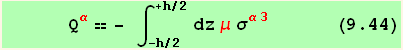
which leads to,
![]()
![]()
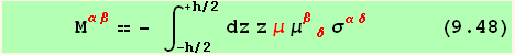
Equation (9.43) differs from the corresponding definition for a plate (7.52) by the presence of the factor ![]() which accounts for the curvature of the shell.
which accounts for the curvature of the shell.
We can do the same treatment for the second term of (9.43). To express the result in the basis ![]() , we use equation (9.1) :
, we use equation (9.1) :

![]()
we define here ![]() (compare with equation (7.52b)),
(compare with equation (7.52b)),

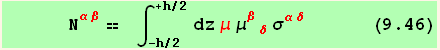
![]()
![]()
And finally the moment (lever arm z ![]() ) of the force dF with respect to the center of the section is,
) of the force dF with respect to the center of the section is,

![]()
![]()
![]()
![]()
Again we define here ![]() (compare with equation (7.52c)),
(compare with equation (7.52c)),

and we have then,
![]()
![]()
The stresses resultants ![]() ,
, ![]() ,
, ![]() have to satisfy differential equations corresponding to the equilibrium of the shell. The treatment is very similar to that in chapter 7, equations
have to satisfy differential equations corresponding to the equilibrium of the shell. The treatment is very similar to that in chapter 7, equations
![]()
![]()
![]()
The 3d covariant derivatives are taken at point B in figure 9.1.
We express these derivatives in terms of 2d covariant derivatives taken in the middle surface.
Starting with ![]() gives,
gives,
![]()
![]()
![]()
![]()
Remark : In the present version of PartialSum we have to use a specific flavor of index β (here blue) to avoid a partial sum also on β.
using (9.18),
![]()
![]()
![]()
![]()
With equation (8.23b) for the 2d covariant derivative we can simplify the above result :
![]()
![]()
![]()
![]()
![]()
![]()
As it will be useful later, we shall multiply this equation by ![]()
![]() . Use of (9.4) (
. Use of (9.4) (![]() ==
==![]()
![]() ==
==![]()
![]() ) and (9.16) gives,
) and (9.16) gives,
![]()
![]()
![]()
![]()
![]()
![]()
![]()
![]()
The first and the last two terms correspond to a 2d covariant derivative.
To simplify the expression, we use the following rule :
![]()
![]()
![]()
![]()
![]()
so that using relation (9.10b),
![]()
![]()

We do the same operations for ![]() , using (9.20) and (8.4) :
, using (9.20) and (8.4) :
![]()
![]()
![]()
![]()
![]()
![]()
![]()
after multiplication by ![]()
![]() and use of (9.4) and (9.2),
and use of (9.4) and (9.2),
![]()
![]()
![]()
![]()
in addition, we have,
![]()
![]()
![]()
![]()
![]()
![]()
![]()
![]()
![]()
Now we come back to equation (9.50), which we also multiply by ![]()
![]() . We obtain,
. We obtain,
![]()
![]()
![]()
![]()
and we integrate this expression via \!\(∫\_\(\(-h\)/2\)\%\(\(+h\)/2\)\)... dz.
![]()
![]()
The first term gives with (9.46):
![]()
![]()
The fourth term gives with (9.44):
![]()
![]()
For the third integral, we use (9.17),
![]()
![]()
This term is the difference of the surface tractions acting on the faces +h/2 and –h/2, each multiplied by a factor which reduces the local metric to that of the middle surface. To that contribution, we can add the first term ∫-h/2+h/2 dz ![]()
![]()
![]() and define,
and define,

The equilibrium condition (equilibrium of forces in the directions ![]() , α =1,2) takes then the form,
, α =1,2) takes then the form,
![]()
![]()
For the equilibrium condition of forces normal to the shell, we start from (6.5), and
![]()
![]()
![]()
![]()
We expand the covariant derivation (chapter 5) of the last term. Then we use equations (9.18), (9.19) and (9.20) to reduce the problem to th middle surface.
The Christoffel symbol ![]() is zero (equation (8.4).
is zero (equation (8.4).
![]()
![]()

![]()
![]()
![]()
![]()
![]()
which allows to eliminate ![]()
![]()
![]()
![]()
In addition, use of equations (9.16) and(9.17) and (8.12)
![]()
![]()
![]()
![]()
![]()
![]()
![]()
![]()
![]()
leads to,
![]()
![]()
We carry over the present results, to (6.5) in chapter 6. We also notice that ![]() ≡
≡ ![]() :
:
![]()
![]()
![]()
then we integrate as before via \!\(∫\_\(\(-h\)/2\)\%\(\(+h\)/2\)\) ...dz
![]()
![]()
this leads to,

![]()
We define,


The final form of the equilibrium condtion for forces normal to the shell is the,
![]()
![]()
Remains the equilibrium of the moments. For that, we insert the factor z in the above expressions. The equation associated with (9.54) gives
![]()
![]()
![]()
![]()
![]()
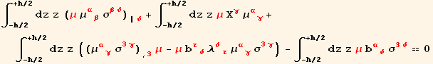
The first term gives with (9.48) (z can be put inside the derivation with respect to δ:
![]()
![]()
For the third integral, after integration by part, we use (9.17),
![]()
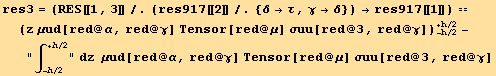
The fourth term gives together with the last term in res3 and with (9.2) and (9.44) :

![]()
and finally the surface tractions and body forces generate the moment,
![]()

The conditions of equilibrium of the moments in the plane tangent to the middle surface are then,
![]()
![]()
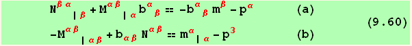
Equations (9.54),(9.56), and(9.58) all issued from (6.4) constitute the three shell conditions which the stress resultants must satisfy.
Other useful but not independent equations, can be derived, in particular the one for the moments about a normal to the shell. We start from the fact that the stress tensor is symmetrical.
![]()
![]()
We apply (9.21) and multiply by μ,
![]()
![]()
![]()
![]()
then we split the factor ![]() using (9.2) (
using (9.2) (![]() ==
==![]() -z
-z ![]() ),
),
![]()
![]()
![]()
![]()
![]()
![]()
![]()
![]()
which gives with (9.46) and (9.48) and changes in the notations of dummy indices (![]() does depend on z),
does depend on z),
![]()
![]()
![]()
![]()
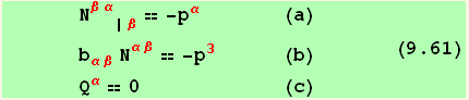
This is a condition imposed to the stress resultants at any single point, which simply represents the symmetry of the stress tensor. It is automatically satisfied via the fundamental shell equations (9.54),(9.56), and (9.58).
Note that using (9.58) we can eliminate the transverse shear force (9.54) and (9.56).
![]()
![]()
![]()
![]()
![]()
![res2 = Eliminate[{res956, CovariantD2d[res958[[1]], red @ α] == 0}, CovariantD2d[Qu[red @ α], red @ α]] ; (*9.6*)](HTMLFiles/index_696.gif)
![]()
It must always kept in mind that the tensors ![]() and
and ![]() are not symmetrical.
are not symmetrical.
It has been shown that for thin enough shells, the contribution to equilibrium of ![]() may be neglected, at least in favorable boundary conditions and absence of discontinuities. In this case
may be neglected, at least in favorable boundary conditions and absence of discontinuities. In this case ![]() must also be absent . The associated theory is called membrane theory.
must also be absent . The associated theory is called membrane theory.
![]()
![]()
![]()
In addition, from (9.59)
![]()
![]()
so that ![]() ==
==![]() . There are only 3 unknowns
. There are only 3 unknowns ![]() ,
,![]() and
and ![]() .
.
Elastic Law
Having established the equilibrium shell conditions (9.54),(9.56), and (9.58), and the kinetic relations (9.34) and (9.40), only one last step remains. We must write the elastic laws which relate the stress resultants with the middle surface strains ![]() and
and ![]() .
.
We start from (9.46) and (9.48), and use Hooke's law (7.21) to express ![]() in terms of strain
in terms of strain ![]() , which we denote now
, which we denote now ![]()
![]()
res721=Tensor[σ, {red[α], Void}, {Void, red[β]}] ==
((Ε*(Tensor[E, {red[α], Void}, {Void, red[β]}] -
(ν*Tensor[g, {red[α], Void}, {Void, red[β]}]*Tensor[E, {red[ζ], Void},
{Void, red[ζ]}])/(-1 + ν)))/(1 + ν)/.{E→η})
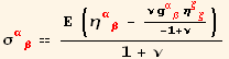
and use of (9.7) after multiplication by ![]() (the rhs is at z = 0),
(the rhs is at z = 0),
![]()
![]()
![]()
![]()
![]()
![]()
![]()
![]()
![]()
![]()
![]()
![]()
We express the strains as covariant components and use (9.7),
![]()

![]()
![]()
![]()
![]()
![]()
![]()
![]()
![]()
![]()
![]()
![]()
![]()
![]()
so that we can now use (9.42),
![]()
![]()
![]()
![resM = res2[[1]] == ((res2Ξ[[2]]/.rul4//Expand//KroneckerAbsorb[a])/.rulλμ//KroneckerAbsorb[g]//Simplify)/.rulinvΞ ; <br />(*9.62*)](HTMLFiles/index_752.gif)
![]()
These equations contain constant terms, ![]() ,
, ![]() , and
, and ![]() , an explicit factor z, and also z- and curvature-dependent terms
, an explicit factor z, and also z- and curvature-dependent terms ![]() ,
, ![]() and
and ![]() . If these terms are explicitly expanded in powers of z, an integration can be performed, and the integration of the even powers (the odd give zero) contain in factor
. If these terms are explicitly expanded in powers of z, an integration can be performed, and the integration of the even powers (the odd give zero) contain in factor
- the extensional stiffness,
![]()
- and the bending stiffness,
![]()
![]()
![]()
![]()
![]()
![]()
![]()
![]()
![]()
![]()
To perform a non symbolic integration, we will use,
![]()
![ruleIntegration[expr_] := (∫_ (-h/2)^(+h/2) (expr/.{Sdz→1, Sbdz→1}) z)](HTMLFiles/index_773.gif)
![]()
![+h/2 ∫ dz f[z] == ∫_ (-h/2)^h/2f[z] z -h/2](HTMLFiles/index_775.gif)
If we neglect all the terms of order ![]() and higher, we have using (9.2), (9.5) and (9.11), after a long and tedious calculation (if done by hand !) ,
and higher, we have using (9.2), (9.5) and (9.11), after a long and tedious calculation (if done by hand !) ,
![]()
![]()
![]()
![]()
![]()

![]()
![]()
![]()
![]()
![]()
![]()
The remaining term below is neglected compared to RESD (two orders in h smaller)
![]()
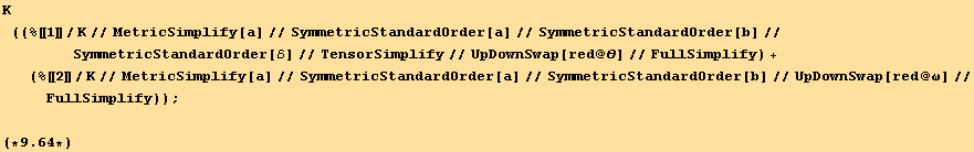
Finally :
![]()
![]()
The treatment of ![]() is completely similar, it only differ by the presence of a factor z in the integrant and a minus sign in the definition (9.48) :
is completely similar, it only differ by the presence of a factor z in the integrant and a minus sign in the definition (9.48) :
![]()
![]()
![]()
![]()
![]()
![]()
![]()
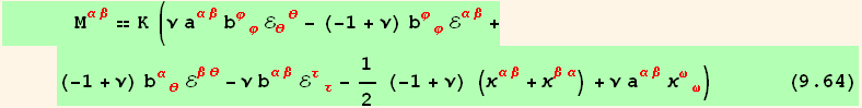
Note : Except for the ![]() term, we find a sign different from equation (9.72) in Flügge's book (?).
term, we find a sign different from equation (9.72) in Flügge's book (?).
The two equations (9.63) and (9.64) represent the elastic law of the shell. Together with the kinematic equations (9.34) and (9.40), and the equilibrium conditions (9.54), (9.56), and (9.58), they are the fundamental equations of shell theory.
![]()
| Created by Mathematica (November 27, 2007) |