10. Elastic Stability

Initialization

Elastic stability

The purpose of this chapter is to consider transitions of elastic structures to to degenerated states of stress. Such a transition, which appears above some critical load, is known as buckling os the structure. This suppose non linear effects in particular the equilibrium condition (6.4) can no more remain linear: In this equation, the stress acts on a volume element considered as undeformed. This is not the case in reality, but when the deformations are small,this approximation is good enough.
    When the load is gradually increased to its critical value, the stresses and the displacements approach everywhere definite limiting values which we denote here by and  .
        As soon as this critical state has been reached, an adjacent state called a buckled state, becomes possible, for which the stress are,

and the displacements,

Formulation of the differential equations of the problem :

As before, we use a coordinate system which is deformed with the body.  In the critical state the base vectors are == with the metric tensor . This will be used as the reference frame

The rectangular body element in figure 10.1 is in the critical state. The face ds×dt on its right-hand side has the area,

Figure 10.1 :

Figure 10.1 Stress acting on a volume element in the prebuckling state.

In the buckled state the base vectors are,

and the force acting is written,

where we still refer to the area before buckling, but using the postbuckling components . The incremental stress is defined by

The force on the right hand side of the volume element may be written,

omiitting the term of higher order.

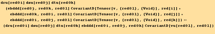
Now, we go back to the derivation of (6.4) for the above volume element. We apply first (6.4) to the stresses before buckling,

where is the volume force then acting. After buckling, the force acting on the pair of faces  ds×dt  of the body is changed by,

The covariant derivative of is zero,
SetScalarSingleCovariantD is added to preserve the covariant derivative of X(= ++ ).

SetScalarSingleCovariantD[False]
rul=CovariantD[Tensor[Tensor[eb, {Void}, {red[m]}]*
   X_], red[i]]→(CovariantD[Tensor[Tensor[eb, {Void}, {red[m]}]*
   Tensor[X]], red[i]]//UnnestTensor//CovariantDSimplify[eb,g,e])

and the same development can be done for the two other pairs of faces, so that the resultant force of all the stresses is,

and this expression can be simplified in a way similar to Chapter 5 (in the Gauss's divergence theorem), which can then be compared to result  ( ) :

so that the resultant force of all the stresses is,

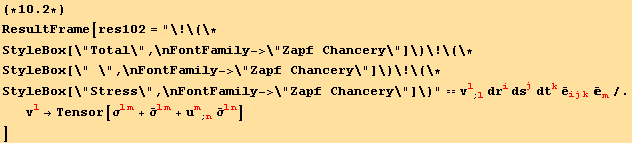
This force is in equilibrium with the body force after buckling,

where is the incremental force.
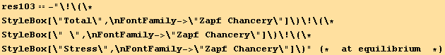
From (10.1), (10.2) and (10.3) we have,

The factor can be droped, and the above relation will be valid for all the coefficients of the so that,

This equation, together with the elastic law (4.3) or (4.11), and the kinematic relation (6.2) applied to the incremental quantities , and are the basic equations of the stability problem.

In the case of gravity forces, as they do not change in magnitude and direction, their incremental load ≡ 0. In the case of centrifugal forces..., the load changes but the increments depend on the buckling deformations and belong to the unknowns of the problem.

Application of equ. (10.4) to the buckling of a plane plate. We suppose the plate loaded by edge forces only (hence ≡ 0), acting in its middle plane. The stress system is that of a plane slab with the stresses uniformly distributed across the thickness (≡0), while ==0.

We introduce the tensor-and-shear tensor , and use all the notations of the plane stress section in Chapter 7:

In the unstable domain, the plate buckles, and each point of the middle plane undergoes a deflection normal to that plane==w, function on but not on =z: points not on the middle plane undergo displacements {w,}, where is given by equation == ==z (equation before equation (7.48) (involving the conservation of the normal).
The incremental strains and stresses are linear functions of z (eqs. (7.48)) and (7.19)). These stresses produce bending and twisting moments (see for instance eq.(7.55)), but no addition to the prebuckling force .

Now, we integrate (10.4) across the plate thickness, for i=3. The integrant is :

In this expression, we note that ==0,=0 :

so that integration of (10.4) reduces to:

The first term gives,

It is zero as there is no stress on the faces of the plate ( ==z),

The term,

vanishes, because of relation (7.9), +====0. It remains,

Using eqs. (7.52a,b), we can relate at equilibrium the transverse shear force produced by the buckling, to the initial plane stress tensor . The curvature   of the buckled plate couples the two.

In a similar manner we can derive a moment equation. The integrant from(10.4) where i→α, is

and the moment equation,

Integrating by parts the first term, and as the stress on the surfaces z=±h/2 is zero,

Using eqs.(7.52c), ==-\!\(∫\_\(\(-\\ h\)/2\)\%\(\(+\\ h\)/2\)\) dz z ,

and for the remaining integrals, we use the kinematic relation  ==z , and again =0

Finally the term do not depend on z, so that

and with the definition of the bending stiffness  K== ,

As shown in Flügge, this contribution RES3 can be neglected. We obtain,

Notice the similarity with equ. (7.57) when =0(external moments absent here).

If we eliminate between (10.5) and (10.6) we find,

To conclude this chapter, let us consider the case of isotropic material. the moments are connected with the deflection w via the same equ. (7.56) as for plate bending.

After differentiation,

Created by Mathematica  (November 27, 2007)